FSP Training 08
Preparation for Mock Exam 09
Instructions
This training page covers all of Section 08 and prepares you for Mock Exam 09. Mock Exam 09 is a full recap in the format of the real FSP: Problem 1 on cost and profit (37 points), Problem 2 on curve sketching with integration (38 points) and Problem 3 on a screening with the binomial distribution (25 points). Set A trains setting up: you translate a text into mathematics and check your translation. It mixes Section 08 with the part types of Mock Exam 09. Set B is a practice mock in the format of Mock Exam 09: 180 minutes plus 5 minutes reading time, 100 points, and all 3 problems must be completed. Write down every step as you would in the exam. The points show what each part is worth.
Keep intermediate results unrounded and type the exact rate per period into the calculator, e.g. \(0.036/12\). Give amounts in EUR to the cent and interest rates in percent with two decimal places. A number of payments or years that must reach a target is rounded up: check the whole numbers on both sides. A payment or an amount that must be reached is a minimum, so round it up to the cent. A largest affordable amount is a maximum, so round it down. A lower limit price is a minimum price: round it up to the cent if you have to round. Round probabilities to four decimal places and other results to two decimal places. A minimum number \(n\) is always rounded up: check \(n - 1\) and \(n\).
In the real FSP, decimals are written with a comma (1,25 means 1.25).
Set A: Set Up & Check (50 minutes)
From Text to Mathematics (xx)
Translate each statement into mathematics. Then answer the check question: it tells you whether your translation works.
A tattoo studio wants to have 9,500 EUR in 3 years for new equipment. Its bank pays 2.25 % per year, compounded monthly. Compute how much the studio must deposit today and write the formula you used.
Check: A classmate says: “Compounding monthly or yearly makes no difference for the deposit.” Compute the amount for yearly compounding and explain the difference.
A company puts 45,000 EUR into a fund that pays 3.5 % per year, compounded continuously. Write the equation for the time after which the capital has grown to 54,000 EUR and solve it. Compute the effective annual rate of the fund.
Check: A classmate solves \(45000 \cdot 1.035^t = 54000\) and gets about 5.30 years. Explain which compounding this equation assumes and why its answer is longer.
A market trader rents a stall in a covered market for 4 years and pays 640 EUR rent at the beginning of each month. The trader calculates with 3 % per year, compounded monthly. Decide which annuity formula fits, write it and compute what the rent payments are worth today.
Check: A classmate answers 30,720 EUR. Explain what this number is and why the value today must be smaller.
A company borrows 48,000 EUR for 5 years at 6.6 % per year, compounded monthly, and repays the loan with equal payments at the end of each month. Compute the monthly payment. Write the first two rows of the amortization schedule (payment, interest, principal, balance).
Check: A classmate computes the interest of the first month as \(48000 \cdot 0.066 = 3{,}168\) EUR. Explain the mistake and check your first row: interest and principal must add up to the payment.
A taxi company wants to buy an electric taxi for 64,000 EUR in 5 years. It deposits the same amount at the end of each month into a savings account that pays 2.9 % per year, compounded monthly. Write the formula for the monthly deposit and compute it.
Check: A colleague divides \(64000 : 60 \approx 1{,}066.67\) EUR. Explain why the correct deposit is smaller, and compute how much of the 64,000 EUR the bank pays as interest.
A workshop makes wooden chopping boards. Its daily costs are \(C(x) = 864 + 15x + 0.06x^2\) in EUR for \(x\) boards. Compute the short-term and the long-term lower limit price. A shop chain pays 21 EUR per board. Decide what the workshop should do in the short run and in the long run.
Check: A colleague says: “21 EUR lies below our lowest unit costs (average total cost), so we must stop production at once.” Explain what is wrong with this argument.
The total costs of a company are a polynomial of third degree, \(C(x) = ax^3 + bx^2 + cx + d\), with \(C\) in MU and \(x\) in QU. Translate each sentence into an equation for \(a\), \(b\), \(c\) and \(d\). Do not solve the system.
(1) The fixed costs are 200 MU.
(2) At 4.5 QU, the curvature of the cost function changes sign (the graph of \(C\) has an inflection point there).
(3) At 3 QU, the marginal costs are 42 MU per QU.
(4) An output of 6 QU costs 560 MU in total.
Check: Show that \(C(x) = 2x^3 - 27x^2 + 150x + 200\) meets all four equations. A classmate writes sentence (2) as \(C'(4.5) = 0\). Explain what this equation would say instead.
An FSP part says: “Determine the nature and the coordinates of all stationary points.” Write the necessary and the sufficient condition you use for \(f(x) = 2x^3 - 9x^2 - 60x + 20\), and carry them out.
Check: A classmate answers: “Maximum at \(x = -2\), minimum at \(x = 5\).” Explain why this answer does not earn full points.
A vet tests cats for a kidney disease with a blood test. 8 % of the tested cats have the disease (\(K\)): this is the prevalence (base rate). The test is positive (\(+\)) for 90 % of the cats with the disease: this is its sensitivity (true positive rate). It is negative (\(-\)) for 94 % of the healthy cats: this is its specificity (true negative rate). Write the three rates as probabilities. Write “a cat with a positive test result does indeed have the disease” and “a cat has the disease but is incorrectly identified as healthy” as probabilities and compute both, e.g. with a table for 2,500 cats.
Check: A classmate writes the specificity as \(P(+ \mid \bar{K}) = 0.94\). Explain what this probability would mean and give its correct value.
In a large call centre, 1.5 % of all calls are cut off by a technical fault, independently of each other. \(X\) is the number of cut-off calls among 600 calls. Write each event with values \(P(X \leq k)\) of the cumulative binomial distribution and compute it with the calculator: (1) not more than 7 calls are cut off, (2) at least 10 calls are cut off, (3) more than 6 but fewer than 12 calls are cut off.
Check: A classmate writes event (3) as \(P(X \leq 12) - P(X \leq 6)\). List the values of \(X\) in the classmate’s event and in event (3).
CautionSolution
Rate per month \(r = \frac{0.0225}{12} = 0.001875\), number of months \(n = 12 \cdot 3 = 36\). Present value (discount the target back to today):
\[PV = 9500 \cdot \left(1 + \frac{0.0225}{12}\right)^{-36} = 9500 \cdot 1.001875^{-36} \approx 8{,}880.4746\]
The studio must deposit at least 8,880.48 EUR (an amount that must be reached is rounded up).
Check: with yearly compounding, the deposit would be \(9500 \cdot 1.0225^{-3} \approx 8{,}886.56\) EUR. With monthly compounding, interest is added every month and earns interest itself, so the money grows faster (\(1.001875^{36} \approx 1.06976 > 1.0225^3 \approx 1.06903\)). A faster-growing deposit needs less money today: 8,880.48 EUR \(<\) 8,886.56 EUR.
Typical mistake: \(9500 \cdot 1.001875^{36}\). This is the value of 9,500 EUR in 3 years, not the amount that grows to 9,500 EUR. Discounting needs the negative exponent.
Continuous compounding: \(A = P e^{rt}\) with \(r = 0.035\):
\[45000 \cdot e^{0.035t} = 54000 \iff e^{0.035t} = 1.2 \iff 0.035t = \ln(1.2) \iff t = \frac{\ln(1.2)}{0.035} \approx 5.21 \text{ years}\]
Effective annual rate: \(r_{\text{eff}} = e^{0.035} - 1 \approx 0.035620\), i.e. 3.56 %.
Check: \(1.035^t\) assumes interest once a year at 3.5 %. Continuous compounding adds interest all the time, which works like 3.56 % once a year. The capital grows faster, so it reaches 54,000 EUR earlier: 5.21 years instead of 5.30 years.
Typical mistake: taking the logarithm before dividing by 45,000 and writing \(\ln(45000 \cdot e^{0.035t}) = 0.035t\). First isolate the power, \(e^{0.035t} = 1.2\), then take the logarithm.
The rent is paid at the beginning of each month, so it is an annuity due. With \(r = \frac{0.03}{12} = 0.0025\) and \(n = 48\):
\[PV_{\text{due}} = PMT \cdot \frac{1 - (1 + r)^{-n}}{r} \cdot (1 + r) = 640 \cdot \frac{1 - 1.0025^{-48}}{0.0025} \cdot 1.0025 \approx 28{,}986.65 \text{ EUR}\]
Check: \(48 \cdot 640 = 30{,}720\) EUR is the total of the payments. A payment in the future is worth less today than its face value, because the money could earn interest until then. Only the first payment is due today, so the value today lies below the total.
Typical mistake: the ordinary annuity formula without the factor \((1 + r)\), which gives about 28,914.36 EUR. It treats every payment as one month later than it really is.
Rate per month \(r = \frac{0.066}{12} = 0.0055\), \(n = 60\) payments. Loan payment:
\[PMT = PV \cdot \frac{r}{1 - (1 + r)^{-n}} = 48000 \cdot \frac{0.0055}{1 - 1.0055^{-60}} \approx 941.4251 \quad \Rightarrow \quad 941.43 \text{ EUR}\]
(rounded up, so that the payments pay off the loan). Schedule: interest = balance \(\cdot\, r\), principal = payment \(-\) interest, new balance = balance \(-\) principal.
Month Payment Interest Principal Balance 0 48,000.00 1 941.43 264.00 677.43 47,322.57 2 941.43 260.27 681.16 46,641.41 Check: 3,168 EUR is the interest of a whole year at 6.6 %. One month carries the rate per period, \(48000 \cdot 0.0055 = 264\) EUR. And \(264.00 + 677.43 = 941.43\) ✓.
Typical mistake: subtracting the whole payment from the balance. Only the principal portion repays the loan, the interest portion is the price of the loan.
Payment from a target value (ordinary annuity, deposits at the end of each month), \(r = \frac{0.029}{12}\), \(n = 60\):
\[PMT = \frac{FV \cdot r}{(1 + r)^n - 1} = \frac{64000 \cdot \frac{0.029}{12}}{\left(1 + \frac{0.029}{12}\right)^{60} - 1} \approx 992.4877 \quad \Rightarrow \quad 992.49 \text{ EUR}\]
(rounded up, so that the target is reached).
Check: the colleague ignores the interest. The deposits earn interest, so they do not have to add up to the whole price. Deposits: \(60 \cdot 992.49 = 59{,}549.40\) EUR, so the bank pays about \(64000 - 59549.40 = 4{,}450.60\) EUR as interest (with the rounded deposit the account reaches 64,000.15 EUR, a few cents more).
Typical mistake: the present value formula \(PV = PMT \cdot \frac{1 - (1 + r)^{-n}}{r}\). The 64,000 EUR are needed at the end, so they are a future value.
Fixed costs \(C_f = 864\), variable costs \(C_v(x) = 15x + 0.06x^2\).
Short-term lower limit price: \(\overline{C}_v(x) = \frac{C(x) - 864}{x} = 15 + 0.06x\) grows with \(x\), so its lowest value is the coefficient of \(x\): 15.00 EUR per board.
Long-term lower limit price: \(\overline{C}(x) = \frac{864}{x} + 15 + 0.06x\), so
\[\overline{C}'(x) = -\frac{864}{x^2} + 0.06 = 0 \iff x^2 = \frac{864}{0.06} = 14{,}400 \iff x = 120 \quad (x > 0)\]
\(\overline{C}''(x) = \frac{1728}{x^3} > 0\), so this is a minimum: \(\overline{C}(120) = 7.20 + 15 + 7.20 = 29.40\) EUR per board.
Decision at 21 EUR: \(15 \leq 21 < 29.40\). In the short run the workshop keeps producing: each board brings in 21 EUR and costs at least 15 EUR in variable costs, so it pays a part of the fixed costs. In the long run the price does not cover the total costs at any output: the workshop needs a higher price or lower costs.
Check: the colleague compares the price only with the long-term lower limit price. Stopping saves only the variable costs, the fixed costs of 864 EUR per day must still be paid. As long as the price lies above the short-term lower limit price of 15 EUR, producing loses less than stopping.
Typical mistake: taking \(\overline{C}_v(120) = 22.20\) EUR as the short-term lower limit price. The short-term lower limit price is the lowest value of \(\overline{C}_v\), not its value at the output with the lowest unit costs.
With \(C'(x) = 3ax^2 + 2bx + c\) and \(C''(x) = 6ax + 2b\):
(1) Fixed costs: \(C(0) = 200\), so \(d = 200\)
(2) The curvature changes sign (inflection point): \(C''(4.5) = 0\), so \(27a + 2b = 0\)
(3) Marginal costs: \(C'(3) = 42\), so \(27a + 6b + c = 42\)
(4) Total costs: \(C(6) = 560\), so \(216a + 36b + 6c + d = 560\)
Check with \(a = 2\), \(b = -27\), \(c = 150\), \(d = 200\): \(54 - 54 = 0\) ✓, \(54 - 162 + 150 = 42\) ✓, \(432 - 972 + 900 + 200 = 560\) ✓. The equation \(C'(4.5) = 0\) would say that the cost function has a horizontal tangent at 4.5 QU, i.e. that one more QU costs nothing there. In fact the marginal costs are lowest there: \(C'(4.5) = 28.5\) MU per QU.
Typical mistake: writing sentence (4) as \(216a + 36b + 6c = 560\). “In total” includes the fixed costs, so \(d\) belongs in the equation.
Necessary condition: \(f'(x) = 0\).
\[f'(x) = 6x^2 - 18x - 60 = 6\left(x^2 - 3x - 10\right) = 6(x - 5)(x + 2) = 0 \iff x = 5 \text{ or } x = -2\]
Sufficient condition: the sign of \(f''(x) = 12x - 18\). \(f''(-2) = -42 < 0\), so \(f\) has a local maximum at \(x = -2\). \(f''(5) = 42 > 0\), so \(f\) has a local minimum at \(x = 5\).
Coordinates: \(f(-2) = -16 - 36 + 120 + 20 = 88\) and \(f(5) = 250 - 225 - 300 + 20 = -255\). Maximum \((-2, 88)\), minimum \((5, -255)\).
Check: “coordinates” asks for both values of each point. The classmate gives only the \(x\)-values and gives no reason (no sufficient condition) for the nature of the points.
Typical mistake: solving \(f(x) = 0\) instead of \(f'(x) = 0\). The zeros of \(f\) are the \(x\)-intercepts, the zeros of \(f'\) are the candidates for stationary points.
Rates: prevalence \(P(K) = 0.08\), sensitivity \(P(+ \mid K) = 0.9\), specificity \(P(- \mid \bar{K}) = 0.94\).
Table for 2,500 cats: \(2500 \cdot 0.08 = 200\) cats with the disease, 2,300 healthy cats.
\(+\) \(-\) sum \(K\) 180 20 200 \(\bar{K}\) 138 2,162 2,300 sum 318 2,182 2,500 Positive result, does indeed have the disease (the base is all positive results): \(P(K \mid +) = \frac{180}{318} \approx 0.5660\)
Has the disease but is incorrectly identified as healthy (one path, the base is all cats): \(P(K \cap -) = 0.08 \cdot 0.1 = \frac{20}{2500} = 0.008\)
Check: \(P(+ \mid \bar{K})\) is the share of the healthy cats that test positive, the false positive rate. It is \(1 - 0.94 = 0.06\): 138 of the 2,300 healthy cats. The specificity is the share of the healthy cats that test negative.
Typical mistake: computing \(P(K \mid -) = \frac{20}{2182}\) for the second question. “Has the disease but is incorrectly identified as healthy” speaks about all tested cats, so it is the joint probability.
\(X \sim B(600;\ 0.015)\). The cumulative function gives \(P(X \leq k)\), so every event is written with such values.
(1) \(P(X \leq 7) \approx 0.3221\)
(2) “At least 10” is the complement of “at most 9”: \(P(X \geq 10) = 1 - P(X \leq 9) \approx 1 - 0.5874 = 0.4126\)
(3) “More than 6 but fewer than 12” means \(X = 7, 8, 9, 10, 11\): \(P(7 \leq X \leq 11) = P(X \leq 11) - P(X \leq 6) \approx 0.8045 - 0.2047 = 0.5998\)
Check: the classmate’s event contains \(X = 7, 8, 9, 10, 11, 12\), event (3) only \(X = 7\) to \(11\). “Fewer than 12” leaves out 12.
Typical mistake: \(P(X \geq 10) = 1 - P(X \leq 10)\). This leaves out \(X = 10\), which belongs to “at least 10”.
One Paragraph, All Conditions (xx)
A company builds electric kilns (ovens for firing clay) and sells them to pottery studios at a fixed market price of 30 MU per QU (1 QU = 10 kilns, 1 MU = 1,000 EUR). Its monthly total costs are a polynomial of third degree in the output \(x\) in QU. The fixed costs are 45 MU. At 9 QU the marginal costs are lowest, at 12 MU per QU. An output of 10 QU costs 311 MU in total. For a new workshop, the company takes out a loan of 240,000 EUR at 5.1 % per year, compounded monthly, and repays it with equal payments at the end of each month over 6 years. The management wants to know the cost function, the output with the lowest unit costs and the long term price floor (the long-term lower limit price), the break-even point and the profit limit (the upper break-even point) at the market price, and the largest monthly profit. It also asks for the monthly loan payment, whether the largest monthly profit covers it, and how much of the loan is still owed after 3 years.
List every given value and every question in this paragraph as a mathematical statement: an equation, a function to minimise or maximise, or a formula. Name the rule or the formula you would use. Do not solve anything.
Check: An assistant writes “At 9 QU the marginal costs are lowest” as \(C'(9) = 0\). Explain what went wrong.
CautionSolution
- Cost function \(C(x) = ax^3 + bx^2 + cx + d\) in MU, \(x\) in QU, with \(C'(x) = 3ax^2 + 2bx + c\) and \(C''(x) = 6ax + 2b\): four unknowns, so four equations
- Fixed costs: \(C(0) = 45\), so \(d = 45\)
- The marginal costs \(C'\) are lowest at 9 QU: the derivative of \(C'\) is zero there, \(C''(9) = 0\) (an inflection point of \(C\))
- Their value there: \(C'(9) = 12\)
- Total costs at 10 QU: \(C(10) = 311\)
- Revenue at the fixed market price: \(R(x) = 30x\), profit \(P(x) = 30x - C(x)\)
- Output with the lowest unit costs: minimise \(\overline{C}(x) = \frac{C(x)}{x}\), i.e. \(\overline{C}'(x) = 0\) (multiplied by \(x^2\), a cubic equation) and \(\overline{C}''(x) > 0\). The long term price floor is the value of \(\overline{C}\) there, in MU per QU (times 100 for EUR per kiln)
- Break-even point and profit limit: the smaller and the larger positive zero of \(P(x) = 0\)
- Largest monthly profit: \(P'(x) = 0\) and \(P''(x) < 0\), then \(P(x)\) in MU (times 1,000 for EUR)
- Loan payment: \(PV = 240{,}000\), \(r = \frac{0.051}{12}\), \(n = 12 \cdot 6 = 72\), \(PMT = PV \cdot \frac{r}{1 - (1 + r)^{-n}}\)
- The profit covers the payment if \(1000 \cdot P_{\max} \geq PMT\)
- Still owed after 3 years: the outstanding balance \(B_{36} = PMT \cdot \frac{1 - (1 + r)^{-36}}{r}\), the present value of the 36 payments that are left
Check: \(C'(9) = 0\) would mean that the costs do not grow at all at 9 QU (a horizontal tangent). “The marginal costs are lowest” is a minimum of \(C'\), so the derivative of \(C'\) is zero: \(C''(9) = 0\). The value of the lowest marginal costs gives a second equation, \(C'(9) = 12\).
Typical mistake: computing the loan payment with \(r = 0.051\) and \(n = 6\). The payments are monthly, so the rate per period is \(\frac{0.051}{12}\) and there are 72 payments.
FSP Words So Far
The FSP problems use these words from Sections 01 to 08. Learn what each one means and how to write it in mathematics.
| Word | Meaning | Mathematics |
|---|---|---|
| quantity unit (QU) | a fixed number of items, e.g. 1 QU = 100 items | the output \(x\) is counted in QU |
| monetary unit (MU) | a fixed amount of money, e.g. 1 MU = 100 EUR | results in MU, convert to EUR at the end |
| fixed costs | costs that arise even if nothing is produced | the constant term of \(C(x)\) |
| variable costs | costs that grow with the output | \(C(x) - C(0)\) (for linear costs: output times costs per QU) |
| total costs | fixed costs + variable costs | \(C(x)\) |
| revenue | quantity times price | \(R(x) = x \cdot \text{price}\) |
| profit | revenue − total costs | \(P(x) = R(x) - C(x)\) |
| break-even point | the output at which the profit changes from negative (a loss) to positive | \(P(x) = 0\), the smaller zero |
| profit limit (upper break-even point) | the larger output with zero profit: above it, the profit turns negative again | \(P(x) = 0\), the larger zero |
| profit zone | all outputs with a positive profit | \(P(x) > 0\): from the break-even point to the profit limit (or the capacity) |
| capacity | the maximum possible output | an upper bound: \(x \leq\) capacity |
| growth factor | the factor by which a quantity is multiplied each period | \(q\) in (starting value) \(\cdot\, q^t\) |
| growth rate | the change per period in percent | \(q = 1 + r\) with \(r\) as a decimal, a loss of 4 % gives \(q = 0.96\) |
| doubling time | the time after which a quantity has doubled | \(q^T = 2\), continuous: \(e^{kT} = 2\), so \(T = \frac{\ln 2}{k}\) |
| half-life (halving time) | the time after which a quantity has halved | \(q^T = 0.5\), continuous: \(e^{-kT} = 0.5\), so \(T = \frac{\ln 2}{k}\) |
| “deviates from \(a\) by at most \(d\)” (tolerance) | the distance from \(a\) is at most \(d\) | \(\lvert x - a \rvert \leq d \iff a - d \leq x \leq a + d\) |
| “share of \(A\) among \(B\)” | the part of \(B\) that also belongs to \(A\): the base is \(B\) | \(\dfrac{\text{number in } A \cap B}{\text{number in } B}\) |
| “neither \(A\) nor \(B\)” | not in \(A\) and not in \(B\), i.e. outside both circles | \(\overline{A \cup B}\) |
| contingency table | a table of counts for two properties: the inner fields are the regions of the Venn diagram, the margins are the totals | inner fields \(A \cap B\), \(A \cap \overline{B}\), \(\overline{A} \cap B\), \(\overline{A} \cap \overline{B}\). Joint probability: field divided by the grand total, conditional probability: field divided by the total of the condition’s row or column |
| gross price, net price | gross price = net price + VAT | with 19 % VAT: gross \(= 1.19 \cdot\) net |
| system of linear equations | several linear equations that must hold at the same time | solve by substitution or elimination, check the solution in every equation |
| no solution, infinitely many solutions | the conditions contradict each other, or one condition only repeats another | elimination leaves \(0 = d\) with \(d \neq 0\), or \(0 = 0\) |
| demand, supply | the quantity buyers want to buy and the quantity sellers offer at a given price | as terms in the price \(p\), e.g. \(Q_d(p)\), \(Q_s(p)\), or as prices \(p_D(x)\), \(p_S(x)\) for the quantity \(x\) |
| market equilibrium | the quantity demanded equals the quantity supplied | demand = supply: \(Q_d(p) = Q_s(p)\), or \(p_D(x) = p_S(x)\). With demand and supply as prices: \(D(q) = S(q)\) gives \(q^*\), and \(p^* = D(q^*)\) |
| price-demand function | gives the price at which \(x\) QU can be sold | \(p(x)\), revenue \(R(x) = x \cdot p(x)\) |
| monopolist | the only supplier of a product, so it can set the price along the demand | its price follows the price-demand function \(p(x)\) |
| average cost (average total cost) | total costs divided by the number of units | \(\overline{C}(x) = \dfrac{C(x)}{x}\) with \(x \neq 0\) |
| zero form | all terms on one side, 0 on the other side | \(ax^2 + bx + c = 0\), then factor or use the quadratic formula |
| discriminant | decides how many real solutions a quadratic equation has | \(\Delta = b^2 - 4ac\): \(> 0\) two, \(= 0\) one, \(< 0\) none |
| biquadratic equation | an equation with only \(x^4\), \(x^2\) and a constant | substitute \(u = x^2\) in \(ax^4 + bx^2 + c\), solve for \(u\), then \(x = \pm\sqrt{u}\) for \(u \geq 0\) |
| domain restrictions (of an equation) | the conditions the unknown must meet so that every term is defined | denominators \(\neq 0\), under a root \(\geq 0\), inside a logarithm \(> 0\) |
| extraneous solution | a candidate that solves the squared equation but not the original one | check every candidate in the original equation |
| function | assigns to every input exactly one output | \(f(x)\), its graph passes the vertical line test |
| domain (of a function) | all inputs for which the function is defined, in a context only the sensible ones | e.g. \([0; \text{capacity}]\) |
| range | all outputs that the function takes on its domain | if the function grows or falls: between the values at the two ends, for a parabola also check the vertex |
| maximum price | the price at which nobody buys any more | \(Q_d(p) = 0\), or \(c\) in \(p = c - dQ\) |
| market saturation | the quantity demanded at a price of 0 | \(a\) in \(Q_d = a - bp\), or the zero of \(p(x)\) |
| shortage, surplus | at a price below the equilibrium price, demand exceeds supply (shortage), above it, supply exceeds demand (surplus) | \(Q_d(p) > Q_s(p)\), or \(Q_d(p) < Q_s(p)\) |
| contribution margin | price minus variable costs per unit: the part of the price that covers the fixed costs | \(p - \overline{C}_v(x)\) per unit. Linear costs: break-even quantity \(= \dfrac{\text{fixed costs}}{\text{contribution margin}}\) |
| vertex | the highest or lowest point of a parabola | \(x_v = -\dfrac{b}{2a}\), or \((h, k)\) in \(a(x - h)^2 + k\) |
| profit-maximizing output | the output with the highest profit | \(x_v\) of \(P(x)\), a maximum since \(a < 0\), and the price \(p(x_v)\). If the capacity lies below \(x_v\): the capacity and its price |
| shift, stretch, compression | moving or scaling a graph | \(a \cdot f(b(x - h)) + k\): first \(b\), then \(h\), then \(a\), then \(k\) |
| mirror image at the \(y\)-axis | the graph flipped from right to left | \(f(-x)\) |
| mirror image at the \(x\)-axis | the graph flipped upside down | \(-f(x)\) |
| composite function | first the inner function, then the outer function | \((f \circ g)(x) = f(g(x))\) |
| inverse function | reverses a function: gives the input that belongs to an output | solve \(y = f(x)\) for \(x\), e.g. \(x(p)\) from \(p(x)\) |
| polynomial of third degree | a function with powers of \(x\) up to \(x^3\) | \(ax^3 + bx^2 + cx + d\) with \(a \neq 0\): four unknowns, so four conditions |
| degree, leading coefficient | the highest power of \(x\), and the number in front of it | together they decide the end behavior |
| zero of multiplicity \(m\) | the factor \((x - c)\) appears \(m\) times in the factored form | odd \(m\): the graph crosses the \(x\)-axis at \(c\), even \(m\): it touches it |
| polynomial long division | divides a polynomial by \((x - c)\) once \(c\) is a known zero | \(f(x) = (x - c) \cdot q(x)\), the remainder must be 0 |
| asymptotic behavior (end behavior) | what happens to \(f(x)\) for \(x \to \infty\) and \(x \to -\infty\) | polynomial: degree and sign of the leading coefficient. Rational function: its asymptotes |
| intercepts | the points where the graph meets the axes | \(y\)-intercept \((0, f(0))\), \(x\)-intercepts from \(f(x) = 0\) |
| rational function | a quotient of two polynomials | \(\dfrac{p(x)}{q(x)}\) with the domain \(q(x) \neq 0\) |
| vertical asymptote | a vertical line near which the values grow without bound | a zero of the denominator that does not cancel |
| hole | a single missing point of the graph | a factor that cancels, its \(y\)-value comes from the simplified term |
| horizontal asymptote | a horizontal line that the graph approaches for \(x \to \pm\infty\) | \(y = c\) with \(f(x) \to c\) |
| oblique asymptote | a slanted line that the graph approaches for \(x \to \pm\infty\) | the linear part of the long division, if the numerator’s degree is one higher |
| grows less than proportionally | grows, but twice the input gives less than twice the output | \(a \cdot x^b\) with \(0 < b < 1\) |
| continuous growth rate | the rate \(k\) of a model with the base \(e\) | \(N_0 \cdot e^{kt}\), growth factor per period \(e^k\) |
| saturation level | a level that a quantity approaches but never exceeds | a horizontal asymptote \(y = L\), e.g. of \(L - a \cdot e^{-kt}\) or \(\dfrac{L}{1 + A e^{-kt}}\) |
| behavior for \(t \to \infty\) | the value a quantity approaches in the long run | \(\lim\limits_{t \to \infty} N(t)\), often with \(e^{-kt} \to 0\) |
| radian | an angle measure in which a full turn is \(2\pi\) | \(180° = \pi\), arc length \(s = r\theta\) |
| amplitude | half the distance between the highest and the lowest value | \(\lvert A \rvert = \dfrac{\max - \min}{2}\) |
| midline | the horizontal line halfway between the highest and the lowest value | \(y = D = \dfrac{\max + \min}{2}\) |
| period | the length of one full cycle | \(B = \dfrac{2\pi}{\text{period}}\) |
| phase shift | the horizontal shift of a sine or cosine curve | \(C\) in \(A\sin(B(t - C)) + D\) or \(A\cos(B(t - C)) + D\) |
| mirror image at the midline | the graph flipped upside down about its midline \(y = D\) | \(2D - f(t)\) |
| limit | the value that \(f(x)\) approaches when \(x\) approaches a number \(a\), or \(\pm\infty\) | \(\lim\limits_{x \to a} f(x)\), one-sided: \(x \to a^-\) (from the left), \(x \to a^+\) (from the right) |
| continuous (at \(a\)) | the graph has no jump and no gap at \(a\) | \(f(a)\) is defined, \(\lim\limits_{x \to a} f(x)\) exists, and both are equal |
| removable discontinuity | a gap that a single value could close, e.g. a hole | the limit exists, but \(f(a)\) is not defined or differs from it |
| derivative | the instantaneous rate of change: the slope of the tangent | \(f'(x) = \lim\limits_{h \to 0} \dfrac{f(x + h) - f(x)}{h}\) |
| secant, slope of the secant | the line through two points of the graph, and its slope (the average rate of change) | \(\dfrac{f(b) - f(a)}{b - a}\) on \([a; b]\) |
| tangent, tangential gradient | the line that touches the graph at a point, and its slope | \(y = f'(a)(x - a) + f(a)\) with the slope \(f'(a)\) |
| angle of intersection (with the \(x\)-axis) | the angle at which a line with slope \(m\) crosses the \(x\)-axis | \(\alpha = \arctan(m)\), with the indicator D for degrees |
| marginal cost, marginal revenue, marginal profit | about the change of the costs, the revenue or the profit caused by one more unit | \(C'(x)\), \(R'(x)\), \(P'(x) = R'(x) - C'(x)\) |
| stationary point (critical point) | a point of the graph with a horizontal tangent | \(f'(x_0) = 0\) |
| nature of a stationary point | whether it is a local maximum, a local minimum or a saddle point | sign change of \(f'\) at \(x_0\), or the sign of \(f''(x_0)\) |
| local maximum, local minimum | a point that is higher (lower) than all points nearby | \(f'(x_0) = 0\) and \(f''(x_0) < 0\) (maximum) or \(f''(x_0) > 0\) (minimum) |
| saddle point | a stationary point at which \(f'\) does not change its sign: the graph levels off and keeps its direction | \(f'(x_0) = 0\) without a sign change, e.g. \(f''(x_0) = 0\) and \(f'''(x_0) \neq 0\) |
| necessary condition, sufficient condition | a condition every candidate must meet, and a condition that proves the kind of point (“prove it really is a maximum”) | necessary: \(f'(x_0) = 0\), sufficient: e.g. \(f''(x_0) < 0\) for a maximum |
| global maximum, global minimum (on an interval) | the highest or lowest value on the whole interval | compare the local extrema with the values at the ends of the interval |
| concave up, concave down | the graph curves upward like a cup, or downward like a cap | \(f''(x) > 0\), or \(f''(x) < 0\) |
| inflection point | the point at which the curvature changes sign: the graph is steepest or flattest there | \(f''(x_0) = 0\) and \(f'''(x_0) \neq 0\), or a sign change of \(f''\) |
| “the curvature changes sign” | the graph changes from concave down to concave up, or back | an inflection point: \(f''(x_0) = 0\). For a cubic cost function, the marginal costs are lowest there |
| inflectional tangent | the tangent at an inflection point: it shows the fastest growth or decline | \(y = f'(a)(x - a) + f(a)\) with \(f''(a) = 0\) |
| unit costs, lowest unit costs | the total costs per unit (the average total cost), and the output at which they are lowest | \(\overline{C}(x) = \dfrac{C(x)}{x}\) (earlier sheets: \(k(x)\)), minimum from \(\overline{C}'(x) = 0\) and \(\overline{C}''(x) > 0\) |
| long term price floor (long-term lower limit price) | the lowest unit costs: below this price, the company cannot cover its total costs in the long run | the minimum value of \(\overline{C}(x) = \dfrac{C(x)}{x}\). Cubic costs: \(\overline{C}'(x) = 0\) times \(x^2\) gives a cubic equation |
| variable costs per unit (variable cost per unit) | the variable costs divided by the output | \(\overline{C}_v(x) = \dfrac{C(x) - C_f}{x}\) (earlier sheets: \(k_v(x)\)) |
| short-term lower limit price | the lowest variable costs per unit: below this price, the company cannot even cover its variable costs | the minimum value of \(\overline{C}_v(x)\). Quadratic costs: the coefficient of \(x\) |
| function family (German: Funktionsschar) | functions with the same term that differ only in a parameter | \(f_a(x)\), e.g. \(f_a(x) = x^2 - ax + 1\) |
| parameter | a letter that is fixed within one function of the family but changes from one function to the next | solve a condition for it, e.g. \(f_a'(2) = 0\) |
| antiderivative (German: Stammfunktion) | a function whose derivative is \(f\) | \(F'(x) = f(x)\) |
| constant of integration | the free constant: two antiderivatives of \(f\) differ only by a constant | \(F(x) + C\), fixed by one condition, e.g. \(C(0) =\) fixed costs or \(P(0) = -\)fixed costs |
| indefinite integral | the family of all antiderivatives | \(\int f(x) \, dx = F(x) + C\) |
| definite integral | a number: the signed area between the graph and the \(x\)-axis from \(a\) to \(b\) | \(\int_a^b f(x) \, dx = F(b) - F(a)\) (Fundamental Theorem of Calculus) |
| lower limit, upper limit | the start \(a\) and the end \(b\) of the interval in \(\int_a^b f(x) \, dx\) | “in the second month”: from \(t = 1\) to \(t = 2\) |
| signed area | area above the \(x\)-axis counts positive, area below it negative | \(\int_a^b f(x) \, dx\), it can be negative or 0 |
| area (between a graph and the \(x\)-axis) | always a positive number | split at the zeros and add the absolute values of the integrals of the pieces |
| net change | the total change of a quantity, computed from its rate of change | \(F(b) - F(a) = \int_a^b F'(x) \, dx\), e.g. extra costs \(\int_a^b C'(x) \, dx\) |
| “total … within the first … months” | everything that has come together from the start up to month \(b\) | \(\int_0^b (\text{rate}) \, dt\) |
| area enclosed by two graphs | the region between the graphs from one intersection point to the next | \(\int_a^b [f(x) - g(x)] \, dx\) with \(f\) on top, limits from \(f(x) = g(x)\), split where the graphs cross |
| “both regions have equal size” | two regions have the same area (not: the integral over both is 0) | compute both areas separately and compare them |
| consumer surplus | what the buyers gain: they would have paid more than the market price | \(CS = \int_0^{q^*} [D(q) - p^*] \, dq\) |
| producer surplus | what the sellers gain: they would have sold for less than the market price | \(PS = \int_0^{q^*} [p^* - S(q)] \, dq\) |
| total surplus | consumer surplus + producer surplus | \(\int_0^{q^*} [D(q) - S(q)] \, dq\), the area between demand and supply |
| minimum price | a price set by the state: no unit may be sold for less | above \(p^*\): only the quantity demanded at this price is traded, and the surpluses end there. Below \(p^*\): no effect |
| average value | the constant height that gives the same area (the same total) over the interval | \(f_{avg} = \frac{1}{b - a}\int_a^b f(x) \, dx\), “average monthly … within the first \(b\) months”: \(\frac{1}{b}\int_0^b f(t) \, dt\) |
| “prove that \(F\) is an antiderivative of \(f\)” | show it by differentiating, no integrating needed | compute \(F'(x)\), e.g. with the product and chain rule, and show \(F'(x) = f(x)\) |
| integration by parts | the integration rule that reverses the product rule | \(\int u \, dv = uv - \int v \, du\), choose \(u\) with LIATE |
| mean | the sum of all values divided by their number | \(\bar{x} = \dfrac{1}{n}\sum x_i\) |
| median | the middle value of the sorted data | odd \(n\): the middle value, even \(n\): the mean of the two middle values |
| quartiles | \(Q_1\) and \(Q_3\): the medians of the lower and the upper half of the sorted data | interquartile range \(\text{IQR} = Q_3 - Q_1\), the middle 50 % of the data. With an odd \(n\), leave the median out of both halves |
| box plot | a picture of the five-number summary | a box from \(Q_1\) to \(Q_3\) with a line at the median, whiskers to the smallest and the largest value that are not outliers |
| outlier | a value far away from the rest of the data | a value outside the fences, i.e. more than \(1.5 \cdot \text{IQR}\) below \(Q_1\) or above \(Q_3\) |
| sample standard deviation | the typical distance of the values of a sample from their mean | \(s = \sqrt{\dfrac{\sum (x_i - \bar{x})^2}{n - 1}}\), for a whole population divide by \(N\) |
| sample space | the set of all possible outcomes of a random experiment | \(S\), e.g. the numbers 1 to 6 for one die |
| event | a set of outcomes | \(A \subseteq S\), with the probability \(P(A)\) between 0 and 1 |
| complement (German: Gegenwahrscheinlichkeit) | “not \(A\)”, everything outside \(A\) | \(P(\bar{A}) = 1 - P(A)\), e.g. “at least one” \(= 1 -\) “none” |
| mutually exclusive | the events cannot happen together | \(A \cap B = \emptyset\), so \(P(A \cup B) = P(A) + P(B)\) |
| independent | one event does not change the probability of the other | \(P(A \cap B) = P(A) \cdot P(B)\), or \(P(A \mid B) = P(A)\), or observed count = expected count |
| “of the …”, “among the …”, “given that …” | names the group that a percentage refers to: the condition | behind the bar: “of the members, 30 % redeem” is \(P(R \mid M) = 0.3\) |
| tree diagram | the stages of a random experiment, with a probability on every branch | the branches that leave one point add up to 1, the second stage carries conditional probabilities |
| path probability | the probability of one path through the tree | multiply along the path (multiplication rule), all path probabilities add up to 1 |
| law of total probability | the probability of an event that several paths lead to | add these paths: \(P(B) = P(A) \cdot P(B \mid A) + P(\bar{A}) \cdot P(B \mid \bar{A})\) |
| Bayes’ theorem | reverses a conditional probability | \(P(A \mid B) = \dfrac{P(A) \cdot P(B \mid A)}{P(B)}\), with \(P(B)\) from the law of total probability |
| base rate (prevalence) | the share of all items (or people) that have the property, before any test | \(P(D)\) |
| true positive rate (sensitivity) | the share of the items with the property that test positive | \(P(+ \mid D)\) |
| true negative rate (specificity) | the share of the items without the property that test negative | \(P(- \mid \bar{D})\) |
| false positive, false negative | a positive result without the property, a negative result with the property | \(\bar{D} \cap +\) and \(D \cap -\), with the rates \(P(+ \mid \bar{D}) = 1 -\) true negative rate and \(P(- \mid D) = 1 -\) true positive rate |
| “… with a positive test result does indeed …” | among the positive results, the ones that are right | the positive predictive value \(P(D \mid +)\), the base is all positive results |
| “… has … but is incorrectly identified as …” | an item has the property, but the test says it has not, seen among all items | the joint probability \(P(D \cap -) = P(D) \cdot P(- \mid D)\), one path of the tree |
| positive predictive value, negative predictive value | the share of the positive results that are right, and the share of the negative results that are right | \(P(D \mid +)\) and \(P(\bar{D} \mid -)\) |
| “Display the fractions in a contingency table. Fill in the blank fields.” | write every given share into its field or total, then complete the table | the fields of a row add up to the row total, the totals add up to the grand total (1 or 100 %) |
| “State the businesslike meaning of the quantities …” | say in words what a set means for the company | e.g. \(\bar{M} \cap R\): “a customer who is not a member and redeems the coupon” |
| expected count | the count of a field if the two properties were independent | \(E = \dfrac{\text{row total} \cdot \text{column total}}{\text{grand total}}\), compare it with the observed count |
| binomial distribution | the number of successes in \(n\) trials | \(P(X = k) = \binom{n}{k} p^k (1 - p)^{n - k}\). Requirements: fixed \(n\), two outcomes per trial, the same \(p\) in every trial, independent trials |
| “exactly / not more than / at least … but not more than …” | which values of \(X\) an event contains | \(P(X = k)\), \(P(X \leq k)\), \(P(a \leq X \leq b)\) with both endpoints. “Fewer than” and “more than” leave out the endpoint |
| expected value | the long-run average of a random variable | \(E[X] = \sum x_i \cdot P(X = x_i)\). Binomial: \(\mu = n \cdot p\) and \(\sigma = \sqrt{n \cdot p \cdot (1 - p)}\) |
| “with a likelihood of at least …” | the probability must reach the given value | \(P(\ldots) \geq\) the value, e.g. for “at least one”: \(1 - \left(1 - p\right)^n \geq\) the value |
| minimum number (of trials) | the smallest whole number \(n\) that meets a condition | solve with logarithms, flip the sign when dividing by \(\ln(1 - p) < 0\), round up and check \(n - 1\) and \(n\) |
| interest rate per period | the rate for one compounding period | \(r = \dfrac{\text{annual rate}}{\text{periods per year}}\), e.g. \(\dfrac{0.036}{12}\) per month |
| compounded monthly / quarterly / continuously | interest is added 12 times or 4 times per year, or all the time | \(A = P\left(1 + \dfrac{r}{n}\right)^{nt}\) with \(n = 12\) or \(n = 4\), continuously \(A = Pe^{rt}\) |
| nominal rate | the annual rate that the bank states, before compounding | \(r\) in \(\dfrac{r}{n}\) |
| effective annual rate (EAR) | the rate that gives the same growth with interest once a year | \(r_{\text{eff}} = \left(1 + \dfrac{r}{n}\right)^n - 1\), continuously \(e^r - 1\). Compare offers by their EAR |
| present value, discount | what a future amount is worth today, and the step from the future back to today | \(PV = FV \cdot (1 + r)^{-t}\) |
| future value | what an amount or a series of payments is worth at a later date | \(FV = PV \cdot (1 + r)^t\) |
| inflation, real interest rate | inflation: the general rise of prices. Real interest rate: the growth of what the money can buy | approximately \(r_{\text{nom}} - r_{\text{infl}}\), exactly \(\dfrac{1 + r_{\text{nom}}}{1 + r_{\text{infl}}} - 1\) |
| annuity, instalment | equal payments at equal time intervals, and one of these payments | \(PMT\) per period, \(n\) payments, rate \(r\) per period |
| ordinary annuity (German: nachschüssig) | payments at the end of each period | \(FV = PMT \cdot \dfrac{(1 + r)^n - 1}{r}\), \(PV = PMT \cdot \dfrac{1 - (1 + r)^{-n}}{r}\) |
| annuity due (German: vorschüssig) | payments at the beginning of each period: each payment earns one period more interest | \(FV_{\text{due}} = FV \cdot (1 + r)\), \(PV_{\text{due}} = PV \cdot (1 + r)\) |
| loan, loan payment | money borrowed now and repaid with equal payments that include the interest | \(PMT = PV \cdot \dfrac{r}{1 - (1 + r)^{-n}}\), total interest \(= n \cdot PMT - PV\) |
| amortization schedule | a table with one row per payment: interest portion, principal portion and balance | interest \(=\) balance \(\cdot\, r\), principal \(= PMT -\) interest, new balance \(=\) balance \(-\) principal |
| principal (two meanings) | (1) the amount borrowed or invested, (2) the part of a payment that repays the loan | (1) \(P\) or \(PV\), (2) the principal portion \(PMT -\) interest |
| outstanding balance | the amount still owed after \(k\) payments | \(B_k = PMT \cdot \dfrac{1 - (1 + r)^{-(n - k)}}{r}\), the present value of the \(n - k\) payments that are left |
| special order | a one-off extra order at a special price, made with spare capacity | with spare capacity: accept if the price lies above the short-term lower limit price (a positive contribution margin), even if it lies below the long term price floor |
In set-builder notation, \(\{x \in \mathbb{R} \mid \dots\}\) and \(\{x \in \mathbb{R} : \dots\}\) mean the same.
Set B: Practice Mock (180 minutes, 100 points)
Problem 1: Massage Chairs for Furniture Stores [37 pts. total]
A company builds massage chairs (armchairs with a built-in massage function) and sells them to furniture stores. An analysis of its monthly costs gives the following information:
- The variable costs per unit (the variable costs divided by the output) are lowest at an output of 14 QU. There they amount to 52 MU per QU.
- At an output of 10 QU, the variable costs per unit are 60 MU per QU.
- At an output of 8 QU, the unit costs (average total cost) are 232 MU per QU.
(1 QU = 100 massage chairs, 1 MU = 1,000 EUR, so a price of \(p\) MU per QU is a price of \(10p\) EUR per chair.)
- Determine the cost function assuming it is a polynomial of third degree. [12 pts.]
Hint: The fixed costs are the constant term \(d\) of \(C\). Write \(\overline{C}_v(x) = \frac{C(x) - d}{x}\) and simplify: you get a polynomial of second degree.
(for verification: \(C(x) = 0.5x^3 - 14x^2 + 150x + 1296\))
- Compute the output volume with the lowest unit costs. Also, determine the long term price floor (the long-term lower limit price) in EUR per massage chair.
Hint: Solve the cubic equation with the polynomial solver (MENU → A → 2, degree 3), or test the whole numbers from 15 to 20.
[5 pts.]
- The stores buy 1,200 massage chairs per month at a price of 1,800 EUR per chair. The market is saturated at 2,100 chairs per month: the stores do not take more chairs, even for free. The demand is linear. Determine the price-demand function \(p(x)\) with \(p\) in MU per QU, and give the maximum price in EUR per chair. [3 pts.]
(for verification: \(p(x) = 420 - 20x\))
Show that the monthly profit is given by \(P(x) = -0.5x^3 - 6x^2 + 270x - 1296\). [2 pts.]
The sales manager claims: “We already make a profit with 500 massage chairs per month, and we stay in the profit zone up to 1,400 chairs.” Determine the break-even point and the profit limit (upper break-even point), and assess both parts of the claim.
Hint: Test the whole numbers from 5 to 8 to find the break-even point.
[6 pts.]
Compute the maximum profit and prove it really is a maximum. [5 pts.]
Calculate the price per massage chair for the maximum profit. A large furniture chain wants to sell the chair under its own brand and offers half of this price, for any number of chairs. Decide whether the company can sign a long-term contract at this price, and whether it should deliver at this price if the contract runs only a few months. [4 pts.]
CautionSolutions
a) Approach: \(C(x) = ax^3 + bx^2 + cx + d\) with the fixed costs \(C_f = d\). Then
\[\overline{C}_v(x) = \frac{C(x) - d}{x} = ax^2 + bx + c, \qquad \overline{C}_v'(x) = 2ax + b, \qquad \overline{C}(x) = \frac{C(x)}{x} = ax^2 + bx + c + \frac{d}{x}\]
Conditions:
- The variable costs per unit are lowest at 14 QU (necessary condition): \(\overline{C}_v'(14) = 0\), so \(28a + b = 0\)
- Their value there: \(\overline{C}_v(14) = 52\), so \(196a + 14b + c = 52\)
- \(\overline{C}_v(10) = 60\), so \(100a + 10b + c = 60\)
- \(\overline{C}(8) = 232\), so \(C(8) = 8 \cdot 232 = 1{,}856\), i.e. \(512a + 64b + 8c + d = 1856\)
Solving:
- From 1: \(b = -28a\)
- 2 minus 3: \(96a + 4b = -8\), so \(96a - 112a = -8\), i.e. \(-16a = -8\) and \(a = 0.5\)
- Back-substitute: \(b = -14\), and from 3: \(50 - 140 + c = 60\), so \(c = 150\)
- From 4: \(256 - 896 + 1200 + d = 1856\), so \(560 + d = 1856\) and \(d = 1296\)
\[C(x) = 0.5x^3 - 14x^2 + 150x + 1296\]
Check: \(\overline{C}_v(x) = 0.5x^2 - 14x + 150\) is a parabola that opens upward with its vertex at \(x = \frac{14}{2 \cdot 0.5} = 14\) and \(\overline{C}_v(14) = 98 - 196 + 150 = 52\) ✓. \(\overline{C}(8) = 32 - 112 + 150 + 162 = 232\) ✓.
Grading: 1 Pt. approach with \(\overline{C}_v(x) = ax^2 + bx + c\), 2 Pts. minimum condition \(\overline{C}_v'(14) = 0\), 1 Pt. \(\overline{C}_v(14) = 52\), 1 Pt. \(\overline{C}_v(10) = 60\), 2 Pts. \(\overline{C}(8) = 232\) turned into \(C(8) = 1{,}856\), 3 Pts. solving the system, 1 Pt. \(C(x)\), 1 Pt. check.
b) Unit costs:
\[\overline{C}(x) = 0.5x^2 - 14x + 150 + \frac{1296}{x}, \qquad \overline{C}'(x) = x - 14 - \frac{1296}{x^2}\]
Necessary condition: \(\overline{C}'(x) = 0\), multiplied by \(x^2 > 0\):
\[x^3 - 14x^2 - 1296 = 0\]
\(x = 18\): \(5832 - 4536 - 1296 = 0\) ✓. There is no other real solution: the long division \((x^3 - 14x^2 + 0x - 1296) : (x - 18) = x^2 + 4x + 72\) leaves a quadratic with the discriminant \(16 - 288 < 0\).
Sufficient condition: \(\overline{C}''(x) = 1 + \frac{2592}{x^3} > 0\) for \(x > 0\), so \(\overline{C}''(18) > 0\): minimum ✓.
The unit costs are lowest at 18 QU = 1,800 massage chairs per month. Long term price floor: \(\overline{C}(18) = 162 - 252 + 150 + 72 = 132\) MU per QU, i.e. 1,320 EUR per massage chair.
Grading: 1 Pt. \(\overline{C}(x)\) and \(\overline{C}'(x)\), 1 Pt. cubic equation, 1 Pt. \(x = 18\) as the only solution, 1 Pt. \(\overline{C}''(18) > 0\), 1 Pt. 1,320 EUR per chair.
c) Points in QU and MU per QU: 1,200 chairs at 1,800 EUR per chair gives \((12, 180)\), the market saturation gives \((21, 0)\).
\[m = \frac{0 - 180}{21 - 12} = -20, \qquad p(x) = -20(x - 21) = 420 - 20x\]
Maximum price: \(p(0) = 420\) MU per QU, i.e. 4,200 EUR per massage chair.
Grading: 1 Pt. both points in QU and MU per QU, 1 Pt. \(p(x)\), 1 Pt. maximum price in EUR.
d) Revenue: \(R(x) = x \cdot p(x) = 420x - 20x^2\)
Profit:
\[P(x) = R(x) - C(x) = 420x - 20x^2 - \left(0.5x^3 - 14x^2 + 150x + 1296\right) = -0.5x^3 - 6x^2 + 270x - 1296 \quad \checkmark\]
Grading: 1 Pt. \(R(x)\), 1 Pt. \(P(x)\) with the bracket resolved correctly.
e) The claim: \(P(5) = -62.5 - 150 + 1350 - 1296 = -158.5 < 0\) and \(P(14) = -1372 - 1176 + 3780 - 1296 = -64 < 0\). At 500 and at 1,400 chairs the company makes a loss.
Break-even point: \(P(6) = -108 - 216 + 1620 - 1296 = 0\) ✓ (and \(P(5) < 0\)), so the break-even point is 6 QU.
Polynomial long division by \((x - 6)\):
\[\begin{array}{l} (-0.5x^3 - 6x^2 + 270x - 1296) : (x - 6) = -0.5x^2 - 9x + 216 \\ \underline{-(-0.5x^3 + 3x^2)} \\ \phantom{(-0.5x^3}\;\; -9x^2 + 270x \\ \phantom{(-0.5x^3}\;\; \underline{-(-9x^2 + 54x)} \\ \phantom{(-0.5x^3 - 9x^2}\;\; 216x - 1296 \\ \phantom{(-0.5x^3 - 9x^2}\;\; \underline{-(216x - 1296)} \\ \phantom{(-0.5x^3 - 9x^2 + 216x - 12}\;\; 0 \end{array}\]
Quadratic formula: \(-0.5x^2 - 9x + 216 = 0 \iff x^2 + 18x - 432 = 0\):
\[x = -9 \pm \sqrt{81 + 432} = -9 \pm \sqrt{513}, \qquad x \approx 13.65 \text{ or } x \approx -31.65\]
The negative solution lies outside the domain. The profit limit is at \(-9 + \sqrt{513} \approx 13.65\) QU.
Profit zone: between the two zeros the profit is positive (test value \(P(10) = 304 > 0\)), so \(6 < x < 13.65\): the company makes a profit with 601 to 1,364 massage chairs per month.
Assessment: both parts of the claim are wrong. The profit starts only above 600 chairs (at 500 chairs the loss is 158,500 EUR), and it ends at about 1,364 chairs (at 1,400 chairs the loss is 64,000 EUR).
Grading: 1 Pt. \(P(5) < 0\) and \(P(14) < 0\), 1 Pt. zero \(x = 6\), 2 Pts. long division, 1 Pt. quadratic formula and profit limit (negative solution excluded), 1 Pt. profit zone and assessment of both claims.
f) Necessary condition:
\[P'(x) = -1.5x^2 - 12x + 270 = 0 \iff x^2 + 8x - 180 = 0 \iff (x - 10)(x + 18) = 0\]
So \(x = 10\) or \(x = -18\) (outside the domain).
Sufficient condition: \(P''(x) = -3x - 12\), so \(P''(10) = -42 < 0\): maximum ✓.
Maximum profit: \(P(10) = -500 - 600 + 2700 - 1296 = 304\) MU, i.e. 304,000 EUR per month with 1,000 massage chairs.
Grading: 1 Pt. \(P'(x)\), 1 Pt. \(x = 10\) (other solution excluded), 1 Pt. \(P''(10) < 0\), 1 Pt. \(P(10) = 304\) MU, 1 Pt. maximum profit in EUR.
g) Price: \(p(10) = 420 - 200 = 220\) MU per QU, i.e. 2,200 EUR per massage chair.
Offer: half of this price is 1,100 EUR per chair.
- Long run: \(1{,}100 < 1{,}320\) EUR, the long term price floor from b). At this price the company cannot cover its total costs at any output, so it cannot accept the price in the long run.
- Short run: the information about the variable costs per unit gives the short-term lower limit price of 52 MU per QU \(= 520\) EUR per chair. \(1{,}100 > 520\) EUR: the price covers the variable costs and pays a part of the fixed costs, so the company should still produce in the short run. Stopping would leave it with the full fixed costs of 1,296,000 EUR per month.
Grading: 1 Pt. price 2,200 EUR, 1 Pt. comparison with the long term price floor, 1 Pt. comparison with the short-term lower limit price, 1 Pt. reason with the fixed costs.
Problem 2: Curve Sketching of an Exponential Function [38 pts. total]
Let the function \(f\) be given by
\[f(x) = \left(x^2 - x - 4\right) \cdot e^{0.25x}, \quad x \in \mathbb{R}\]
Round all results to two decimal places.
State the domain of \(f\). Determine the \(x\)- and \(y\)-intercepts of \(G_f\). [3 pts.]
Investigate the asymptotic behavior of \(f\). Give the equation of the asymptote and state from which side \(G_f\) approaches it. [3 pts.]
Determine the first and the second derivative of \(f\). [4 pts.]
(for verification: \(f'(x) = 0.25(x - 1)(x + 8) \cdot e^{0.25x}\) and \(f''(x) = \frac{1}{16}\left(x^2 + 15x + 20\right) \cdot e^{0.25x}\))
Determine the nature and the coordinates of all stationary points. [7 pts.]
Assess how many inflection points \(f\) has to possess at least. Give a reason for your answer. Then compute the inflection points. [4 pts.]
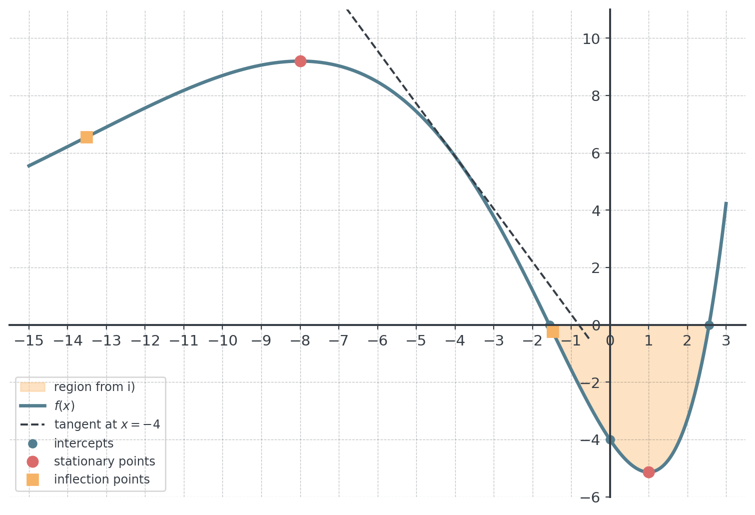
Determine the tangent of \(f\) at \(x = -4\). [3 pts.]
Sketch the graph \(G_f\) in the interval \([-15; 3]\). Draw the tangent from f) into the same figure. [5 pts.]
Find the antiderivative of \(f(x)\) and show your work. [5 pts.]
(for verification: \(F(x) = \left(4x^2 - 36x + 128\right) \cdot e^{0.25x}\))
- \(G_f\) and the \(x\)-axis enclose a region below the \(x\)-axis. Mark the region in your sketch and compute its area. Explain why the integral of \(f\) from one zero to the other is not the area itself. [4 pts.]
CautionSolutions
a) Domain: the polynomial and \(e^{0.25x}\) are defined for every real number, so \(D_f = \mathbb{R}\).
\(y\)-intercept: \(f(0) = (-4) \cdot e^0 = -4\), i.e. \((0, -4)\).
\(x\)-intercepts: \(e^{0.25x} > 0\) for every \(x\), so only the bracket can become zero:
\[x^2 - x - 4 = 0 \iff x = \frac{1 \pm \sqrt{1 + 16}}{2} = \frac{1 \pm \sqrt{17}}{2}, \qquad x_1 \approx -1.56, \quad x_2 \approx 2.56\]
i.e. \((-1.56, 0)\) and \((2.56, 0)\).
Grading: 1 Pt. domain, 1 Pt. \(y\)-intercept, 1 Pt. \(x\)-intercepts with the reason \(e^{0.25x} > 0\).
b) \(x \to \infty\): \(x^2 - x - 4 \to \infty\) and \(e^{0.25x} \to \infty\), so \(\lim\limits_{x \to \infty} f(x) = \infty\).
\(x \to -\infty\): \(e^{0.25x} \to 0\), and the exponential beats the power: with \(t = -x\), \(x^2 \cdot e^{0.25x} = t^2 \cdot e^{-0.25t} \to 0\) for \(t \to \infty\), and the same holds for \(x \cdot e^{0.25x}\) and \(e^{0.25x}\). So \(\lim\limits_{x \to -\infty} f(x) = 0\).
Asymptote: \(y = 0\) (the \(x\)-axis), only for \(x \to -\infty\). For \(x < x_1 \approx -1.56\) the bracket is positive, so \(f(x) > 0\): \(G_f\) approaches the \(x\)-axis from above.
Grading: 1 Pt. limit for \(x \to \infty\), 1 Pt. limit for \(x \to -\infty\) with the reason, 1 Pt. asymptote \(y = 0\) on the left, approached from above.
c) First derivative (product rule, and the chain rule for \(e^{0.25x}\)): \(u = x^2 - x - 4\), \(v = e^{0.25x}\), \(u' = 2x - 1\), \(v' = 0.25e^{0.25x}\).
\[f'(x) = (2x - 1) \cdot e^{0.25x} + \left(x^2 - x - 4\right) \cdot 0.25e^{0.25x} = \left(0.25x^2 + 1.75x - 2\right) \cdot e^{0.25x} = 0.25(x - 1)(x + 8) \cdot e^{0.25x}\]
Second derivative (product rule on \(f'(x) = \left(0.25x^2 + 1.75x - 2\right) \cdot e^{0.25x}\), with \(u' = 0.5x + 1.75\)):
\[f''(x) = (0.5x + 1.75) \cdot e^{0.25x} + \left(0.25x^2 + 1.75x - 2\right) \cdot 0.25e^{0.25x} = \left(0.0625x^2 + 0.9375x + 1.25\right) \cdot e^{0.25x} = \frac{1}{16}\left(x^2 + 15x + 20\right) \cdot e^{0.25x}\]
Grading: 1 Pt. \(u\), \(v\), \(u'\), \(v'\) with the chain rule, 1 Pt. \(f'(x)\) factored, 1 Pt. product rule for \(f''\), 1 Pt. \(f''(x)\) factored.
d) Necessary condition: \(f'(x) = 0\). Since \(0.25e^{0.25x} \neq 0\):
\[(x - 1)(x + 8) = 0 \iff x = 1 \text{ or } x = -8\]
Sufficient condition:
- \(f''(1) = \frac{1}{16}(1 + 15 + 20) \cdot e^{0.25} = 2.25e^{0.25} > 0\): local minimum
- \(f''(-8) = \frac{1}{16}(64 - 120 + 20) \cdot e^{-2} = -2.25e^{-2} < 0\): local maximum
Coordinates: \(f(1) = -4e^{0.25} \approx -5.14\) and \(f(-8) = 68e^{-2} \approx 9.20\). Local minimum at \((1, -5.14)\), local maximum at \((-8, 9.20)\).
Grading: 1 Pt. necessary condition with \(e^{0.25x} \neq 0\), 1 Pt. both \(x\)-values, 2 Pts. sufficient condition at both points, 1 Pt. nature of both points, 2 Pts. coordinates.
e) Assessment: at the maximum, \(G_f\) is concave down (\(f''(-8) < 0\)), at the minimum it is concave up (\(f''(1) > 0\)). So the curvature changes its sign at least once between \(-8\) and \(1\). Left of the maximum, \(G_f\) comes from the \(x\)-axis (approached from above, part b) and rises to the maximum. To level off towards the asymptote far to the left, it must be concave up there, but it is concave down at the maximum. So the curvature changes its sign a second time left of \(-8\): \(f\) has at least two inflection points.
Computation: \(f''(x) = 0\). Since \(\frac{1}{16}e^{0.25x} \neq 0\):
\[x^2 + 15x + 20 = 0 \iff x = \frac{-15 \pm \sqrt{225 - 80}}{2} = \frac{-15 \pm \sqrt{145}}{2}, \qquad x_3 \approx -13.52, \quad x_4 \approx -1.48\]
Both are simple zeros of \(f''\), so \(f''\) changes its sign there. Inflection points \((-13.52, 6.55)\) and \((-1.48, -0.23)\).
Grading: 2 Pts. assessment with both reasons, 1 Pt. both \(x\)-values, 1 Pt. sign change and coordinates.
f) Point and slope: \(f(-4) = (16 + 4 - 4) \cdot e^{-1} = 16e^{-1} \approx 5.89\) and \(f'(-4) = 0.25 \cdot (-5) \cdot (-4 + 8) \cdot e^{-1} = -5e^{-1} \approx -1.84\).
\[t(x) = f'(-4) \cdot (x + 4) + f(-4) = -5e^{-1}(x + 4) + 16e^{-1} = -\frac{5x + 4}{e} \approx -1.84x - 1.47\]
Grading: 1 Pt. \(f(-4)\), 1 Pt. \(f'(-4)\), 1 Pt. tangent equation.
g) Table of values (rounded to two decimal places):
| \(x\) | \(-15\) | \(-13\) | \(-11\) | \(-9\) | \(-8\) | \(-6\) | \(-4\) | \(-2\) | \(-1\) | \(0\) | \(1\) | \(2\) | \(3\) |
|---|---|---|---|---|---|---|---|---|---|---|---|---|---|
| \(f(x)\) | \(5.55\) | \(6.90\) | \(8.18\) | \(9.06\) | \(9.20\) | \(8.48\) | \(5.89\) | \(1.21\) | \(-1.56\) | \(-4\) | \(-5.14\) | \(-3.30\) | \(4.23\) |
Grading: 1 Pt. labelled axes and a suitable scale on \([-15; 3]\), 1 Pt. intercepts and stationary points, 1 Pt. inflection points with the correct curvature, 1 Pt. flat approach to the \(x\)-axis from above on the left and steep rise on the right, 1 Pt. tangent.
h) Integration by parts, \(\int u \, v' \, dx = u \cdot v - \int u' \cdot v \, dx\), twice. With \(v' = e^{0.25x}\) we get \(v = 4e^{0.25x}\).
First step: \(u = x^2 - x - 4\), \(u' = 2x - 1\):
\[\int \left(x^2 - x - 4\right) e^{0.25x} \, dx = 4\left(x^2 - x - 4\right) e^{0.25x} - 4\int (2x - 1) \, e^{0.25x} \, dx\]
Second step: \(u = 2x - 1\), \(u' = 2\):
\[\int (2x - 1) \, e^{0.25x} \, dx = 4(2x - 1) \, e^{0.25x} - \int 8e^{0.25x} \, dx = 4(2x - 1) \, e^{0.25x} - 32e^{0.25x}\]
Together:
\[F(x) = e^{0.25x}\left[4x^2 - 4x - 16 - 16(2x - 1) + 128\right] = \left(4x^2 - 36x + 128\right) \cdot e^{0.25x} \; (+\, C)\]
Check: \(F'(x) = (8x - 36)e^{0.25x} + \left(4x^2 - 36x + 128\right) \cdot 0.25e^{0.25x} = \left(x^2 - x - 4\right) e^{0.25x} = f(x)\) ✓
Grading: 1 Pt. choice of \(u\) and \(v'\) with \(v = 4e^{0.25x}\), 1 Pt. first integration by parts, 1 Pt. second integration by parts, 1 Pt. \(\int 8e^{0.25x} \, dx = 32e^{0.25x}\), 1 Pt. \(F(x)\) simplified.
i) Between the zeros \(x_1 = \frac{1 - \sqrt{17}}{2} \approx -1.5616\) and \(x_2 = \frac{1 + \sqrt{17}}{2} \approx 2.5616\), the bracket \(x^2 - x - 4\) is negative, so \(f(x) < 0\): the region lies below the \(x\)-axis.
\[\int_{x_1}^{x_2} f(x) \, dx = F(x_2) - F(x_1) \approx 117.68 - 131.28 = -13.59\]
(with the unrounded values \(F(x_2) \approx 117.6850\) and \(F(x_1) \approx 131.2775\)). The area is \(A \approx 13.59\) area units.
Explanation: below the \(x\)-axis the integral counts the region negatively (signed area), so it gives \(-13.59\). An area is never negative, so the area is the absolute value of the integral.
Grading: 1 Pt. limits \(x_1\) and \(x_2\) with \(f < 0\) between them, 1 Pt. \(F(x_2)\) and \(F(x_1)\), 1 Pt. area 13.59, 1 Pt. explanation.
Problem 3: Testing Blood Donations [25 pts. total]
A regional blood donation service collects 50,000 blood donations per year. Every donation is tested for the hepatitis E virus with a quick test. Donations with a positive test result (\(+\)) are discarded, donations with a negative result (\(-\)) go to the hospitals. Let \(V\) be the event “the donation contains the virus”. The prevalence (base rate) of the virus among the donations is 0.4 %. The test’s sensitivity (true positive rate) is 98 %, its specificity (true negative rate) is 99.5 %.
- Create a tree diagram for the testing and complete the following table for the 50,000 donations of one year. [6 pts.]
| positive (\(+\)) | negative (\(-\)) | sum | |
|---|---|---|---|
| contains the virus (\(V\)) | |||
| free of the virus (\(\bar{V}\)) | |||
| sum | 50,000 |
(for verification: 445 of the 50,000 donations test positive)
Compute the probability that a donation is free of the virus but is incorrectly identified as infected. Give the number of donations per year that are discarded although they are free of the virus. [3 pts.]
The head of the laboratory says: “Our test finds 98 % of the infected donations, so 98 % of the discarded donations really contain the virus.” Compute the probability that a donation with a positive test result does indeed contain the virus, and assess the statement. [4 pts.]
Determine the number of donations which need to be tested to find at least one infected donation testing positive with a likelihood (probability) of 99 %. [4 pts.]
In one week, the service tests 700 donations. Compute the probability for the following events:
(1) Exactly 7 donations test positive.
(2) Not more than 5 donations test positive.
(3) At least 6 but not more than 10 donations test positive.
(4) More than 12 donations test positive.
[8 pts.]
CautionSolutions
a) Given: \(P(V) = 0.004\) (prevalence), \(P(+ \mid V) = 0.98\) (sensitivity), \(P(- \mid \bar{V}) = 0.995\) (specificity). Complements: \(P(\bar{V}) = 0.996\), \(P(- \mid V) = 0.02\) (false negative rate), \(P(+ \mid \bar{V}) = 0.005\) (false positive rate).
Tree diagram (first stage: virus or not, second stage: test result, path probability = product along the path):
- \(V\) (\(0.004\)) \(\to\) \(+\) (\(0.98\)): \(0.00392\), \(\quad V \to -\) (\(0.02\)): \(0.00008\)
- \(\bar{V}\) (\(0.996\)) \(\to\) \(+\) (\(0.005\)): \(0.00498\), \(\quad \bar{V} \to -\) (\(0.995\)): \(0.99102\)
Check: \(0.00392 + 0.00008 + 0.00498 + 0.99102 = 1\) ✓
Table (path probability \(\cdot\) 50,000):
| \(+\) | \(-\) | sum | |
|---|---|---|---|
| \(V\) | 196 | 4 | 200 |
| \(\bar{V}\) | 249 | 49,551 | 49,800 |
| sum | 445 | 49,555 | 50,000 |
Check: \(200 + 49{,}800 = 445 + 49{,}555 = 50{,}000\) ✓
Grading: 2 Pts. tree diagram with the complements, 3 Pts. inner fields and totals, 1 Pt. check.
b) Joint probability, the base is all 50,000 donations (one path of the tree):
\[P(\bar{V} \cap +) = P(\bar{V}) \cdot P(+ \mid \bar{V}) = 0.996 \cdot 0.005 = 0.00498 = \frac{249}{50000}\]
So 249 donations per year are discarded although they are free of the virus.
Grading: 1 Pt. joint probability with the base 50,000, 1 Pt. value, 1 Pt. 249 donations.
c) Positive predictive value, the base is all 445 donations with a positive result (Bayes’ theorem):
\[P(V \mid +) = \frac{P(V) \cdot P(+ \mid V)}{P(+)} = \frac{0.00392}{0.00392 + 0.00498} = \frac{196}{445} \approx 0.4404 = 44.04\,\%\]
Assessment: the statement is wrong. 98 % is the sensitivity \(P(+ \mid V)\), its base is the infected donations. The share of infected donations among the discarded ones is \(P(V \mid +) \approx 44.04\,\%\), with the discarded donations as the base. The virus is rare (0.4 %), so the 0.5 % false positives among the 49,800 donations without the virus (249) outnumber the 196 infected donations that the test finds. More than half of the discarded donations are free of the virus.
Grading: 1 Pt. base 445 (Bayes’ theorem), 1 Pt. result, 2 Pts. assessment with the two bases and the low prevalence.
d) A tested donation contains the virus and tests positive with \(p = P(V \cap +) = 0.00392\) (from a). Complement: “at least one” \(= 1 -\) “none”:
\[1 - 0.99608^n \geq 0.99 \iff 0.99608^n \leq 0.01\]
Logarithm: \(n \cdot \ln(0.99608) \leq \ln(0.01)\). Since \(\ln(0.99608) < 0\), dividing by it reverses the sign:
\[n \geq \frac{\ln(0.01)}{\ln(0.99608)} \approx \frac{-4.6052}{-0.0039277} \approx 1172.48\]
Round up: 1,173 donations. Check: \(1 - 0.99608^{1172} \approx 0.98998 < 0.99\), but \(1 - 0.99608^{1173} \approx 0.99002 \geq 0.99\) ✓.
Grading: 1 Pt. \(p = 0.00392\) (the joint probability, not the sensitivity), 1 Pt. complement inequality and logarithm, 1 Pt. sign reversal, 1 Pt. rounding up with the check.
e) \(X\) = number of donations with a positive result among the 700 donations. Each donation tests positive with \(P(+) = \frac{445}{50000} = 0.0089\) from a), independently of the others, so \(X \sim B(700;\ 0.0089)\):
\[P(X = k) = \binom{700}{k} \cdot 0.0089^k \cdot 0.9911^{700 - k}\]
(1) Exactly 7:
\[P(X = 7) = \binom{700}{7} \cdot 0.0089^7 \cdot 0.9911^{693} \approx 0.1430\]
Events (2) to (4) have many terms, so use the cumulative distribution \(P(X \leq x)\) of the calculator.
Calculator: MENU → 7 → ▼ → 1 → 2 (Variable), then x, N = 700 and p = 0,0089, each with =, and = again gives \(P(X \leq x)\). For \(P(X = x)\), use MENU → 7 → 4 (Binomial-Dichte) → 2 in the same way.
(2) Not more than 5 (0 to 5):
\[P(X \leq 5) \approx 0.4086\]
(3) At least 6 but not more than 10 (both endpoints included, so \(X \leq 5\) is taken away):
\[P(6 \leq X \leq 10) = P(X \leq 10) - P(X \leq 5) \approx 0.9479 - 0.4086 = 0.5393\]
(4) More than 12 (13 or more), with the complement:
\[P(X \geq 13) = 1 - P(X \leq 12) \approx 1 - 0.9886 = 0.0114\]
Grading: 2 Pts. binomial model with \(n = 700\) and \(p = 0.0089\) from a), 1 Pt. exactly 7, 1 Pt. not more than 5, 2 Pts. between 6 and 10 as \(P(X \leq 10) - P(X \leq 5)\), 2 Pts. more than 12 as \(1 - P(X \leq 12)\).
Exam Preparation Checklist
Before the exam, check that you can:
Show all work, name the base of every probability, and interpret your results in the business context.