Session 04-02 - Power, Root & Rational Functions
Section 04: Advanced Functions
Entry Quiz
Review from Session 04-01
Work individually for 5 minutes, then we discuss
Determine the end behavior of \(P(x) = -3x^4 + 2x^2 - 7\)
Given \(Q(x) = 2(x - 1)^3(x + 2)\), identify all zeros and their multiplicities and describe what they mean
If a polynomial has degree 5, what is the maximal number of turning points it can have?
Sketch \((x - 2)(x + 1)^2\) on a number line
Homework Discussion
Your questions from Tasks 04-01
Focus on polynomial applications and factoring
- Challenges with the Rational Root Theorem
- Sketching polynomials from factored form
- Interpreting multiplicity in graphs
- Business context questions
Power functions will help us understand the individual components of polynomials!
Learning Objectives
Today’s Goals
By the end of this session, you will be able to:
- Understand power functions with integer, fractional, and negative exponents
- Determine domains of root functions and fractional powers
- Sketch power function graphs without a calculator
- Compare growth rates of different power functions
- Apply power functions to economic models
- Analyze rational functions (asymptotes, holes) and average-cost models
Integer Powers
Definition and Basic Forms
The building blocks of polynomials
A power function has the form \[f(x) = ax^n \quad (a \neq 0,\; n \text{ real})\]
- Integer powers: \(x^2, x^3, x^{-1}, x^{-2}\)
- Root functions: \(\sqrt{x}, \sqrt[3]{x}\)
- Fractional powers: \(x^{2/3}, x^{3/2}\)
Simpler than polynomials, but they reveal behaviors that explain all functions.
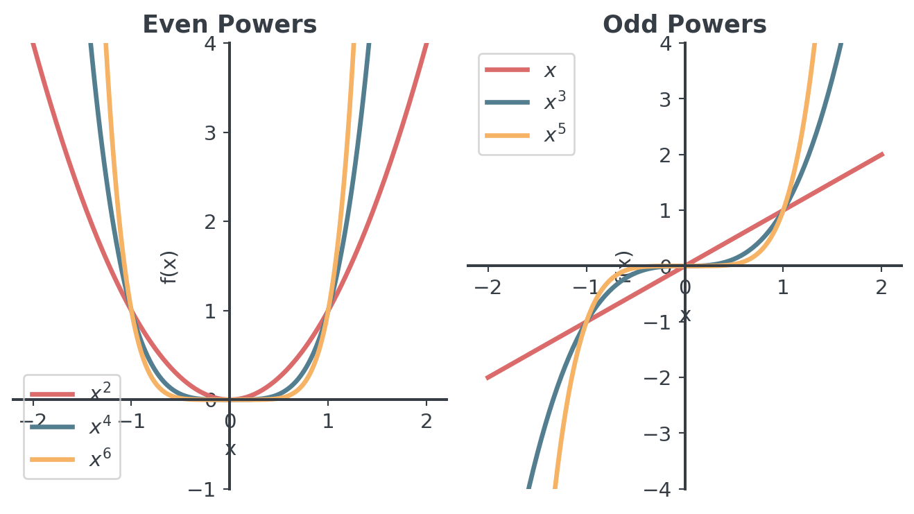
Comparing even and odd powers
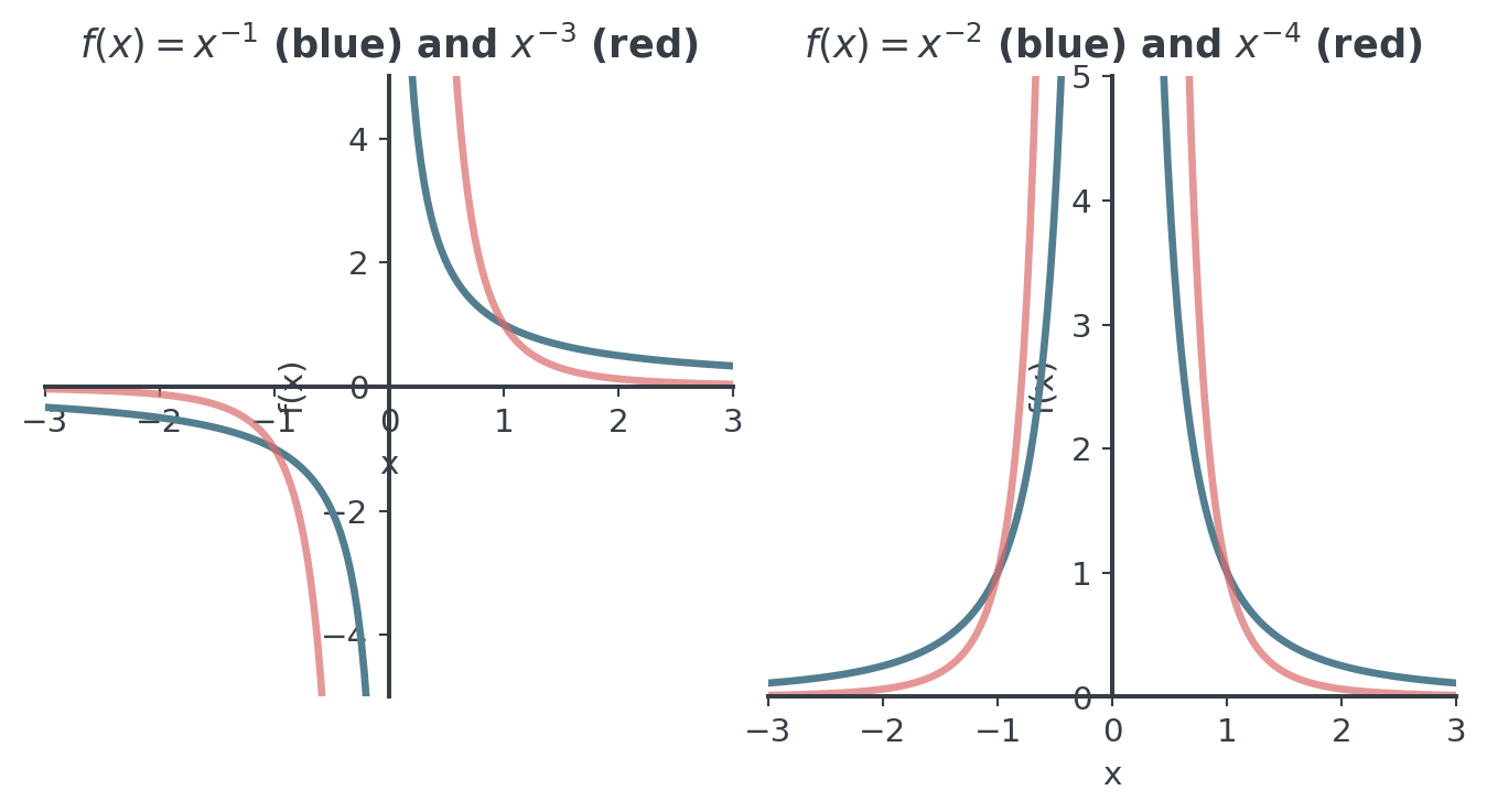
Negative Integer Powers
For \(n > 0\): \(f(x) = x^{-n} = \frac{1}{x^n}\), not defined at \(x = 0\)
Root Functions
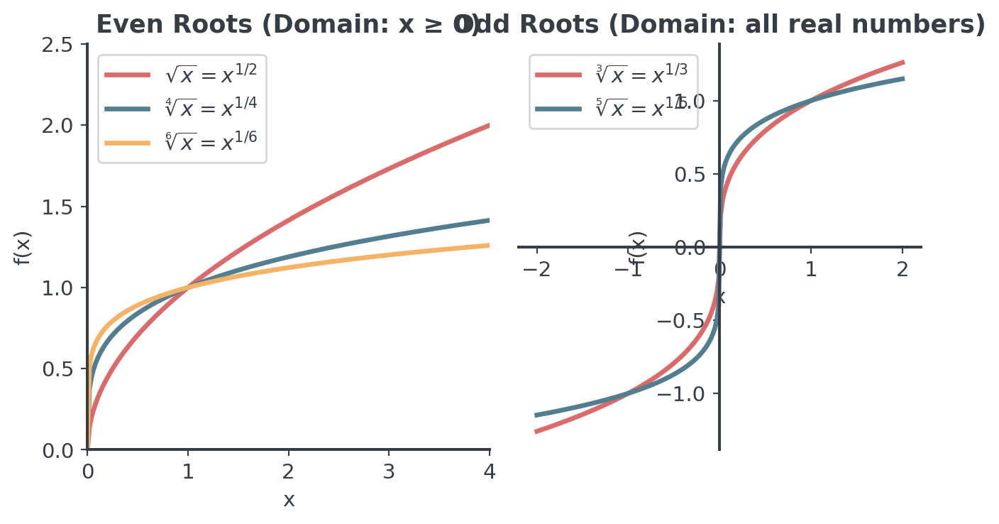
Functions with fractional exponents
Domain Restrictions
Critical concept for root functions
like \(\sqrt{x}\), \(\sqrt[4]{x}\):
- Domain: \(x \geq 0\) only
- Why? Even roots of negative numbers aren’t real
- \(\sqrt{x^2} = |x|\) (always non-negative)
- Range: \(y \geq 0\)
like \(\sqrt[3]{x}\), \(\sqrt[5]{x}\):
- Domain: all real numbers
- Can take cube root of negative numbers
- Range: all real numbers
Fractional Powers
General Fractional Exponents
Combining powers and roots
For \(f(x) = x^{m/n}\) where \(m, n\) are integers, \(n > 0\):
\[x^{m/n} = (x^{1/n})^m = \sqrt[n]{x^m}\]
Domain depends on \(n\):
- If \(n\) is odd: all real numbers (usually)
- If \(n\) is even: \(x \geq 0\) required
Example: \(f(x) = x^{3/2} = \sqrt{x^3} = (\sqrt{x})^3\)
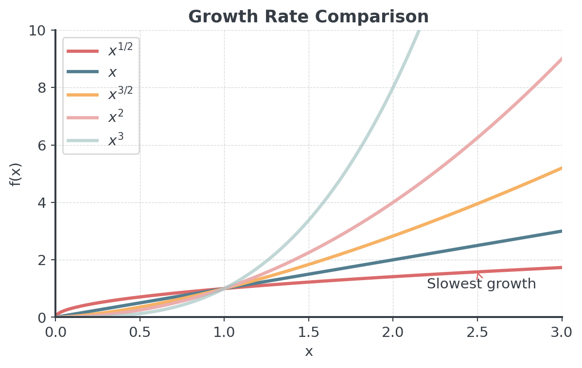
- Domain: \(x \geq 0\) (because of square root), grows faster than \(\sqrt{x}\) but slower than \(x^2\)
Comparing Growth Rates
Economic Applications
Economies of Scale
Cost functions with fractional powers
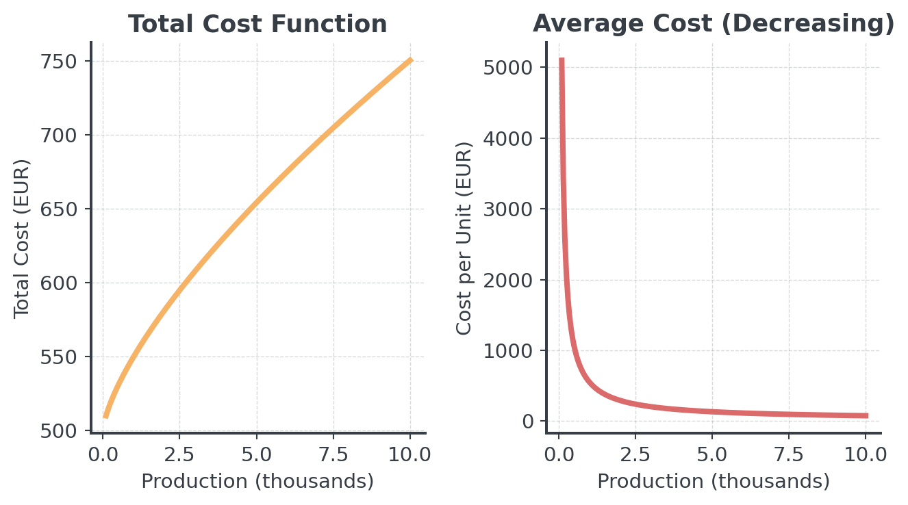
Many production processes exhibit economies of scale:
\[C(x) = 500 + 50x^{0.7}\]
where \(x\) is production quantity (thousands)
Question: Any idea why \(x^{0.7}\)?
Exponent < 1 means cost grows slower than production!
Economies of Scale II
Allometric Growth I
Biological and economic scaling
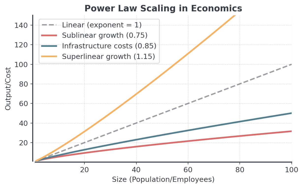
Many relationships follow power laws:
- Biology: Brain mass ∝ (Body mass)\(^{0.75}\)
- Economics:
- City infrastructure costs ∝ (Population)\(^{0.85}\)
- Company revenue ∝ (Number of employees)\(^{1.15}\)
Have you ever seen ∝ before? That’s the proportionality symbol (∝), which means “is proportional to” in mathematics.
Allometric Growth II
Area & Volume
Geometric Power Relationships
Why packaging costs don’t scale linearly
Example: Doubling box dimensions
- Surface area increases by factor of \(2^2 = 4\)
- Volume increases by factor of \(2^3 = 8\)
- Material cost (surface) vs. capacity (volume)
This explains why larger packages have lower cost per unit volume. The discount has a mathematical basis!
Graphing Techniques
Sketching Power Functions
A systematic approach
Steps to sketch \(f(x) = ax^n\) or \(f(x) = ax^{m/n}\):
Determine domain
- Negative exponents: exclude \(x = 0\)
- Even roots: require \(x \geq 0\)
Find key points
- Always passes through \((1, a)\) if in domain
- Check \((0, 0)\) if applicable
Analyze end behavior
- Positive exponents: consider even/odd
- Negative exponents: approach axes
Check symmetry
- Even exponents: y-axis symmetry
- Odd exponents: origin symmetry
Practice: Sketch Without Calculator
Work together
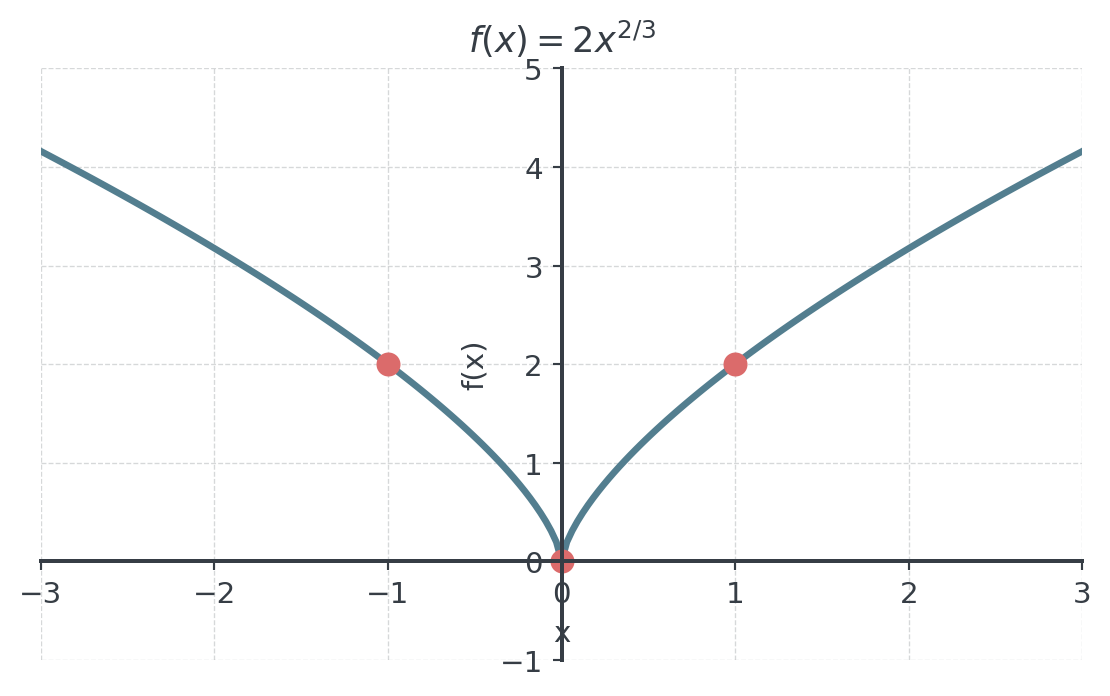
Sketch: \(f(x) = 2x^{2/3}\)
Sketch: The Result
Practice Domain & Range Analysis
Work together and discuss
For each function, determine the domain and range, then sketch a rough graph:
\(f(x) = 3x^{1/4}\)
\(g(x) = -2x^{-1}\)
\(h(x) = x^{3/5}\)
\(p(x) = 4 - x^{1/2}\)
Break
Combining Powers
Sums and Products
Building complex models
Real-world phenomena often combine power functions:
Total Cost with Multiple Effects:
\[C(x) = 1000x^{0.5} + 50x + 0.1x^2\]
- \(x^{0.5}\): Setup costs (economies of scale)
- \(x\): Linear variable costs
- \(x^2\): Capacity constraints (diseconomies)
Rational Functions
Structure of Rational Functions
A rational function has the form:
\(f(x) = \frac{P(x)}{Q(x)}\), where \(P(x)\) and \(Q(x)\) are polynomials and \(Q(x) \neq 0\)
- Domain: All real numbers except where \(Q(x) = 0\)
- Zeros: Where \(P(x) = 0\) (and \(Q(x) \neq 0\))
- Vertical Asymptotes: Where \(Q(x) = 0\) (canceling common factors)
- Holes: Where both \(P(x) = 0\) and \(Q(x) = 0\) (canceled factors)
- Horizontal/Oblique Asymptotes: Determined by degree comparison
What Are Asymptotes?
An asymptote is a line a function approaches
- Think of it like a boundary the graph gets infinitely close to
- Vertical asymptotes: Never crossed or touched (undefined there)
- Horizontal/oblique asymptotes: Can be crossed at finite x-values, but approached as \(x \to \pm\infty\)
- Three types: vertical, horizontal, and oblique (slanted)
Vertical Asymptotes
Occur where the denominator equals zero (and numerator doesn’t)
Mathematical definition: \[\lim_{x \to a^-} f(x) = \pm\infty \quad \text{or} \quad \lim_{x \to a^+} f(x) = \pm\infty\]
- The function “blows up” (goes to \(\infty\) or \(-\infty\))
- Graph has a vertical line at \(x = a\)
- Function is undefined at this point
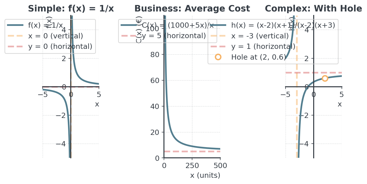
- Example: \(f(x) = \frac{1}{x}\) has vertical asymptote at \(x = 0\)
Horizontal Asymptotes
Three cases, based on the degrees of \(P(x)\) and \(Q(x)\)
\[f(x) = \frac{2x + 1}{x^3 - 5}\]
- Denominator grows faster
- Horizontal asymptote: \(y = 0\)
- The function approaches zero
\[f(x) = \frac{3x^2 + 2x - 1}{2x^2 + 5}\]
- Both grow at same rate
- Horizontal asymptote: \(y = \frac{3}{2}\) (ratio of leading coefficients)
\[f(x) = \frac{x^3 + 2x}{x^2 - 1}\]
- Numerator grows faster
- No horizontal asymptote
- May have an oblique (slanted) asymptote instead
Oblique (Slanted) Asymptotes
When degree of P exceeds degree of Q by exactly 1
- Perform polynomial long division (as in 04-01): \(\frac{P(x)}{Q(x)} = L(x) + \frac{R(x)}{Q(x)}\)
- The quotient \(L(x)\) (a linear function) is the oblique asymptote
- As \(x \to \pm\infty\), the remainder term \(\frac{R(x)}{Q(x)} \to 0\)
Example: \(f(x) = \frac{x^2 + 1}{x - 1} = x + 1 + \frac{2}{x-1}\)
Oblique asymptote: \(y = x + 1\)
Holes vs. Asymptotes
Critical distinction when factors cancel!
- Factor appears in both numerator and denominator
- Example: \(f(x) = \frac{(x-2)(x+1)}{(x-2)(x+3)}\)
- Factor \((x-2)\) cancels: hole at \(x = 2\), not an asymptote!
- Simplified: \(f(x) = \frac{x+1}{x+3}\), \(x \neq 2\)
- Factor appears only in denominator
- \(f(x) = \frac{x+1}{x+3}\)
- Factor \((x+3)\) doesn’t cancel
- Vertical asymptote at \(x = -3\)
- Function undefined, goes to \(\pm\infty\)
Always factor completely and cancel common factors before identifying asymptotes!
Examples for Rational Functions
Asymptote Rules
Systematic Approach for Finding Asymptotes
Step 1: Factor completely \[f(x) = \frac{P(x)}{Q(x)} = \frac{\text{factored form}}{\text{factored form}}\]
Step 2: Cancel common factors → These create holes
Step 3: Vertical asymptotes → Remaining factors in denominator
Step 4: Horizontal/Oblique asymptotes → Compare degrees
Asymptote Analysis Challenge
3 minutes individual, 2 minutes pair discussion, 2 minutes class share
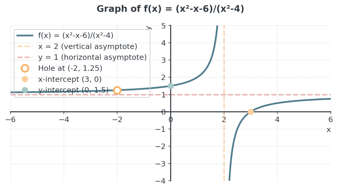
Analyze the function: \(f(x) = \frac{x^2 - x - 6}{x^2 - 4}\)
Your tasks:
- Factor numerator and denominator
- Identify any holes
- Find all asymptotes
- Determine x and y intercepts
- Sketch a rough graph
Asymptote Analysis
Average Cost
Average Cost Functions
In business, the average cost per unit is:
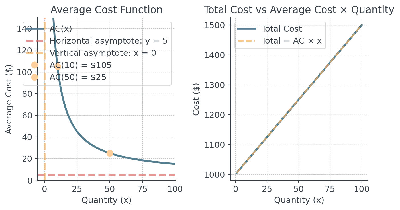
\[AC(x) = \frac{\text{Total Cost}}{\text{Quantity}} = \frac{C(x)}{x} = \frac{F + vx}{x} = \frac{F}{x} + v\]
- \(F\) = Fixed costs
- \(v\) = Variable cost per unit
- \(x\) = Number of units
Do you get the idea here?
Key Properties
These functions often have the same properties:
- Vertical asymptote at \(x = 0\)
- Horizontal asymptote at \(y = v\)
- Always decreasing for \(x > 0\) (economies of scale)
- Average cost stays above \(v\) and approaches it as \(x \to \infty\)
Let’s see an example!
Visualization of Average Cost
Manufacturing Analysis
Work through this business scenario and then we compare
A company has fixed costs of 5000 EUR per month and variable costs of 20 EUR per unit.
- Write the average cost function
- Find the horizontal asymptote and interpret it
Manufacturing Analysis II
- How many units bring average cost to within 5 EUR of the asymptote?
- Graph the function
Hint for c): The denominator is positive, so you can multiply both sides by it without changing the sign.
Guided Practice
Individual Exercise Block I
Work alone for 5 minutes, then discuss for 5 minutes
Problem 1: A company’s profit function combines multiple effects: \[P(x) = -2x^3 + 15x^2 + 100\sqrt{x} - 500\]
where \(x\) is production level (hundreds of units), \(x > 0\)
- Identify each term’s economic interpretation
- Calculate \(P(4)\) and \(P(9)\)
- Which term dominates for large \(x\)? What does this tell management?
Individual Exercise Block II
Work alone for 5 minutes, then discuss for 5 minutes
Problem 2: Compare growth rates for large values:
- Which grows faster: \(f(x) = x^{1/2}\) or \(g(x) = x^{1/3}\)?
- Which grows faster: \(f(x) = x^{3/2}\) or \(g(x) = x^2\)?
- Order from slowest to fastest growth: \(x^{1/2}, x, x^{3/2}, x^2\)
Individual Exercise Block III
Work alone for 5 minutes, then discuss for 5 minutes
Problem 3: A technology company’s average cost per unit is: \[AC(x) = \frac{50000}{x} + 100 + 0.01x\]
where \(x\) is units produced.
- Identify the power function in each term
- What happens to average cost as \(x \to 0^+\) (positive \(x\) near 0)?
- What happens to average cost as \(x \to \infty\)?
- Graph the behavior conceptually
Spot the Error
Can you find what’s wrong? Work with your neighbor
Time allocation: 5 minutes to find errors, 5 minutes to discuss
Student work:
“\(\sqrt{x^2} = x\) for all \(x\)”
“The function \(f(x) = x^{-1/2}\) has domain \(x > 0\)”
“Since \(x^{2/3} = \sqrt[3]{x^2}\), the domain is \(x \geq 0\)”
“\(x^{1.5}\) grows faster than \(x^2\) because 1.5 is complicated”
Not everything has to be wrong!
Coffee Break
FSP Workshop
Problem 1: Inspection Queue
A company runs a vehicle inspection station with one inspection lane. An inspection takes 3 minutes on average, so the lane can handle at most 20 cars per hour. If on average \(x\) cars arrive per hour, the company’s planning model gives the average time a car spends at the station (waiting plus inspection) as
\[T(x) = \frac{60}{20 - x} \text{ minutes.}\]
- Give the domain of \(T\) in this context and interpret \(T(0)\). Determine the vertical asymptote of \(T\) and explain its meaning for the station. [4 pts.]
Inspection: Busy Hours
Give the range of \(T\) on its domain. The station manager says: “If arrivals rise by 20 %, from 15 to 18 cars per hour, the time at the station also rises by about 20 %.” Assess this statement. [3 pts.]
The station promises: “On average, you are back on the road within 15 minutes.” Determine all arrival rates for which the promise holds. [3 pts.]
Hint: Dividing the same positive number by a smaller positive number gives a larger result. In c), the denominator is positive, so you can multiply both sides by it without changing the sign.
Inspection: A Faster Device
A new test device cuts the inspection to 2 minutes, so the lane can handle at most 30 cars per hour. The model becomes \(T_2(x) = \frac{60}{30 - x}\).
- Show that \(T_2(x) = T(x - 10)\). Describe the transformation and give the new vertical asymptote. Determine, with the transformation, all arrival rates for which the 15-minute promise now holds. [4 pts.]
Inspection: Does It Pay?
- Each inspection brings a margin of 40 EUR (fee minus variable costs). The station is open 40 hours per week, and enough customers would come. It always works at the largest arrival rate that keeps the promise. The device costs 2,400 EUR per week. Decide whether it pays off. [2 pts.]
Wrap-Up & Takeaways
Key Takeaways
Today’s essential concepts
- Power functions are the building blocks of polynomials
- Domain restrictions come from mathematical necessity
- Growth rate comparisons guide long-term planning
- Fractional powers create realistic economic models
Final Assessment
5 minutes - Individual work
A manufacturing company’s cost per unit follows: \[C(x) = 10000x^{-0.5} + 50 + 2x^{0.5}\] where \(x\) is the number of units produced (in thousands).
What is the domain of this function in the business context?
Identify each term’s economic meaning
What happens to cost per unit as production increases dramatically?
Which term represents economies of scale?
Next Session Preview
Session 04-03: Exponential & Logarithmic Functions
Moving from power to exponential growth
- Exponential growth and decay, doubling time and half-life
- The natural exponential \(e^x\), compound interest, continuous growth
- Exponential vs. power function growth (critical comparison!)
- Logarithmic functions, semi-log and log-log scales
Complete Tasks 04-02!