Session 05-06 - Optimization & Curve Sketching

Section 05: Differential Calculus

Entry Quiz - 10 Minutes

Quick Review from Session 05-05

Test your understanding of limits, continuity, and function families

1. For \(f_t(x) = x^2 - 4tx + 3\), find \(t\) such that \(f_t(x)\) has exactly one zero.

2. Evaluate \(\lim_{x \to 4} \frac{x^2 - 16}{x - 4}\)

3. Is \(f(x) = \begin{cases} x + 2 & x < 1 \\ 3 & x = 1 \\ 2x & x > 1 \end{cases}\) continuous at \(x = 1\)?

4. Find \(\lim_{n \to \infty} \frac{3n^2 + 5n}{2n^2 - 1}\)

Homework Discussion - 15 Minutes

Your questions from Session 05-05

What questions do you have regarding the previous session?

Learning Objectives

What You’ll Master Today

• Apply the first derivative test to classify critical points
• Use the second derivative test when applicable
• Find global extrema on closed intervals
• Master the complete curve sketching algorithm (6 steps)
• Solve optimization problems in business contexts
• Maximize profit and minimize cost using calculus
• Sketch complete, accurate graphs of functions

. . .

Optimization is the central application of calculus in business! Today’s techniques will help you maximize profit, minimize cost, and make optimal decisions.

Part A: Derivative Tests for Extrema

Critical Points Review

A critical point of \(f(x)\) occurs at \(x = c\) if:

• \(f'(c) = 0\) (horizontal tangent), OR
• \(f'(c)\) does not exist (sharp corner, vertical tangent, etc.)

. . .

Key Fact: Extrema (max/min) can only occur at:

1. Critical points (inside the domain)
2. Endpoints of the domain
3. Points where \(f\) is not differentiable

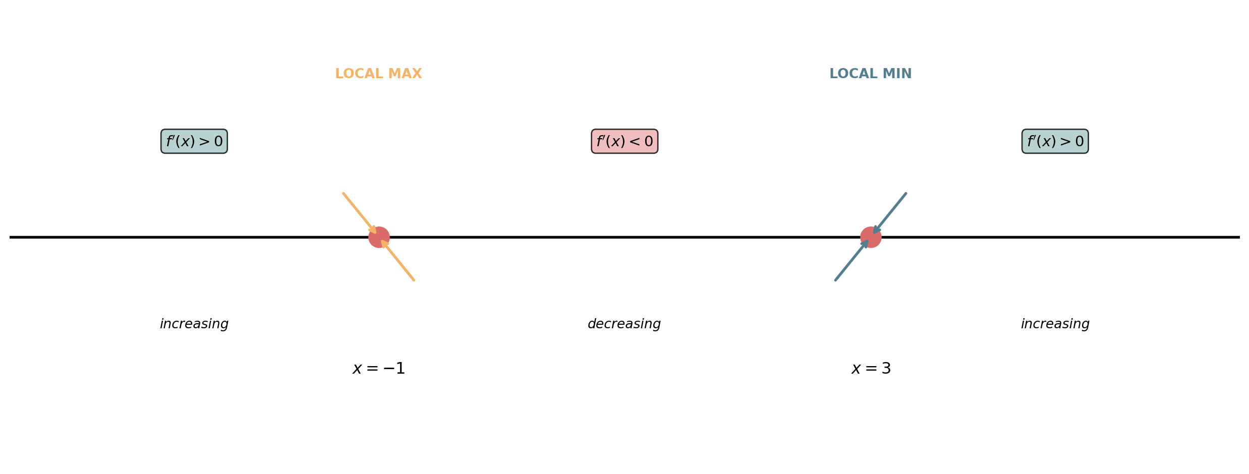
First Derivative Test

To classify a critical point at \(x = c\), examine how \(f'(x)\) changes sign:

1. Local Maximum: If \(f'\) changes from \((+)\) to \((-)\) at \(x = c\)
   • Function increases before \(c\), decreases after \(c\)
2. Local Minimum: If \(f'\) changes from \((-)\) to \((+)\) at \(x = c\)
   • Function decreases before \(c\), increases after \(c\)
3. Neither (Inflection): If \(f'\) does not change sign at \(x = c\)
   • Example: \(f(x) = x^3\) at \(x = 0\)

First Derivative Test Example

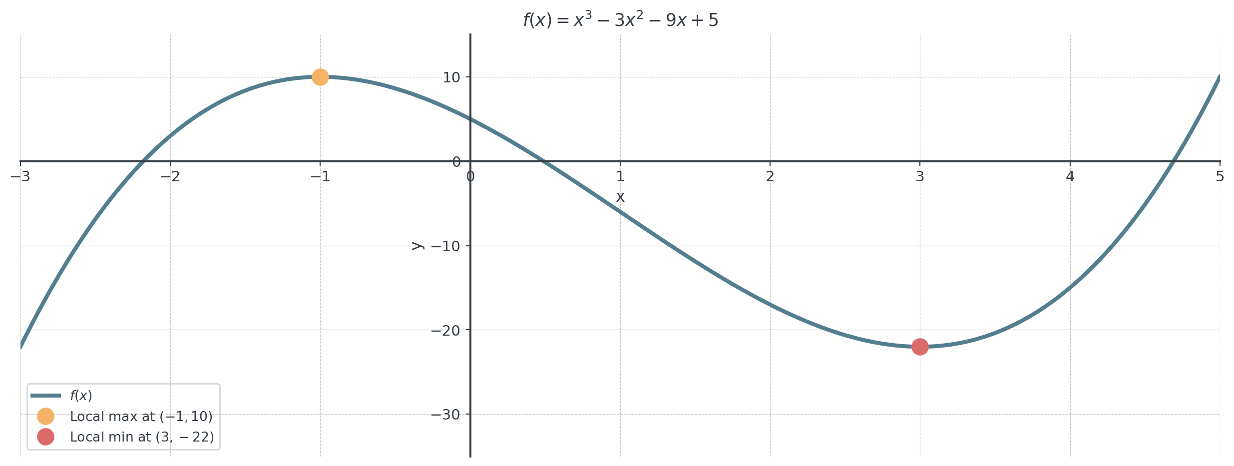
Problem: Find and classify all critical points of \(f(x) = x^3 - 3x^2 - 9x + 5\).

. . .

Step 1: Find \(f'(x)\): \[f'(x) = 3x^2 - 6x - 9 = 3(x^2 - 2x - 3) = 3(x-3)(x+1)\]

. . .

Step 2: Find critical points (\(f'(x) = 0\)): \[x = -1 \text{ or } x = 3\]

. . .

Step 3: Create a sign chart for \(f'(x)\):

Sign Chart Analysis

• \(f'\) changes from \((+)\) to \((-)\) at \(x = -1\) → Local maximum
• \(f'\) changes from \((-)\) to \((+)\) at \(x = 3\) → Local minimum

Visualizing the Function

. . .

Makes intuitive sense, doesn’t it?

Second Derivative Test

Alternative Method: If \(f'(c) = 0\) and \(f''(c)\) exists:

1. If \(f''(c) > 0\): The function is concave up at \(c\) → Local minimum
   • Think: holding water (bottom of a bowl)
2. If \(f''(c) < 0\): The function is concave down at \(c\) → Local maximum
   • Think: shedding water (top of a hill)
3. If \(f''(c) = 0\): The test is inconclusive → Use first derivative test

. . .

WarningWhen to Use Which Test?

• First derivative test: Always works, requires sign chart
• Second derivative test: Faster when \(f''\) is easy to compute, but can be inconclusive

Second Derivative Test Example

Problem: Use on \(f(x) = x^3 - 3x^2 - 9x + 5\) at \(x = -1\) and \(x = 3\).

. . .

Find \(f''(x)\): \[f''(x) = 6x - 6\]

. . .

At \(x = -1\): Local maximum \[f''(-1) = 6(-1) - 6 = -12 < 0\]

. . .

At \(x = 3\): Local minimum \[f''(3) = 6(3) - 6 = 12 > 0\]

When Second Derivative Test Fails

Example: \(f(x) = x^4\)

• \(f'(x) = 4x^3\), so \(f'(0) = 0\) (critical point at \(x = 0\))
• \(f''(x) = 12x^2\), so \(f''(0) = 0\) (inconclusive!)

. . .

Use first derivative test instead:

• For \(x < 0\): \(f'(x) = 4x^3 < 0\) (decreasing)
• For \(x > 0\): \(f'(x) = 4x^3 > 0\) (increasing)
• Sign changes from \((-)\) to \((+)\) → Local minimum at \(x = 0\)

Part B: Global Extrema on Intervals

Extreme Value Theorem

If \(f\) is continuous on closed interval \([a, b]\), then \(f\) has both:

• An absolute maximum (global max)
• An absolute minimum (global min)

. . .

Strategy to find global extrema on \([a, b]\):

1. Find all critical points \(c\) in \((a, b)\)
2. Evaluate \(f\) at all critical points
3. Evaluate \(f\) at both endpoints: \(f(a)\) and \(f(b)\)
4. Largest value = absolute maximum
5. Smallest value = absolute minimum

Example: Global Extrema

Challenge: Find the absolute maximum and minimum of \(f(x) = x^3 - 3x + 2\) on \([-2, 2]\).

. . .

Step 1: Find critical points.

. . .

\[f'(x) = 3x^2 - 3 = 3(x^2 - 1) = 3(x-1)(x+1) = 0\]

. . .

\[x = -1 \text{ or } x = 1\]

. . .

Both are in \((-2, 2)\)

. . .

Step 2: Evaluate \(f\) at critical points and endpoints.

Evaluation Table

\(x\)	\(f(x) = x^3 - 3x + 2\)	Type
\(-2\)	\((-2)^3 - 3(-2) + 2 = -8 + 6 + 2 = 0\)	Endpoint
\(-1\)	\((-1)^3 - 3(-1) + 2 = -1 + 3 + 2 = 4\)	Critical
\(1\)	\((1)^3 - 3(1) + 2 = 1 - 3 + 2 = 0\)	Critical
\(2\)	\((2)^3 - 3(2) + 2 = 8 - 6 + 2 = 4\)	Endpoint

. . .

Common exam mistake: Finding critical points but forgetting to check endpoints.

• The global maximum/minimum might occur at \(x = a\) or \(x = b\)
• Always create a table comparing ALL candidates (critical points + endpoints)
• In business: Production constraints define your “endpoints”

Visualizing Global Extrema

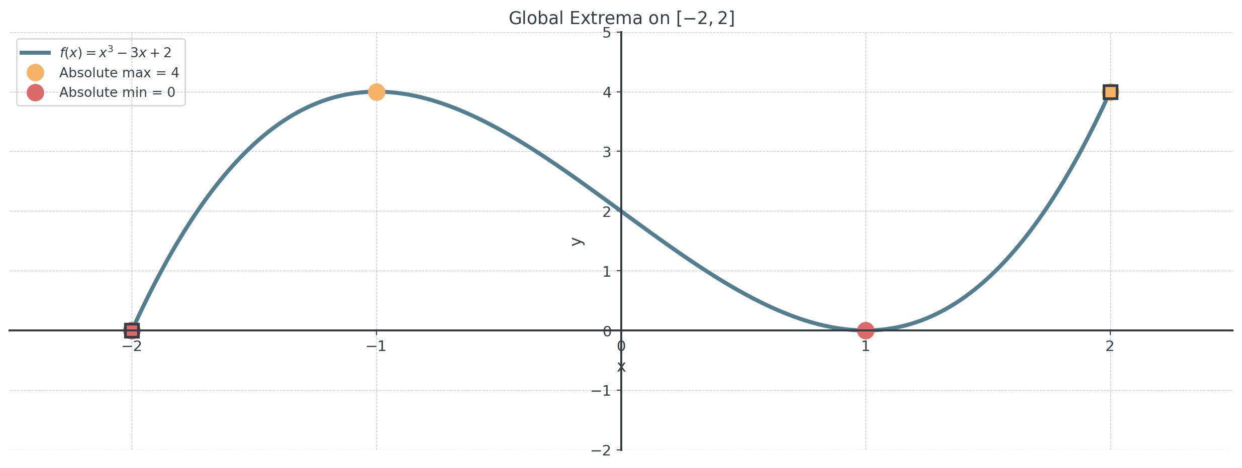
• Squares indicate the interval endpoints
• Circles show where extrema occur

Quick Practice - 10 Minutes

Practice Problems

Work individually, then compare with a neighbor

1. Find all critical points of \(g(x) = x^4 - 4x^3 + 5\).

2. Use the second derivative test to classify the critical points of \(g(x)\) from problem 1.

3. Find the absolute maximum and minimum of \(h(x) = x^2 - 4x + 1\) on \([0, 5]\).

4. For \(f(x) = 2x^3 - 3x^2 - 12x + 7\), use the first derivative test to classify all critical points.

Break - 10 Minutes

Part C: Complete Curve Sketching Algorithm

The 6-Step Algorithm

Master Process for Sketching \(y = f(x)\):

1. Domain and Intercepts
   • Find where \(f\) is defined
   • \(y\)-intercept: \(f(0)\)
   • \(x\)-intercepts: solve \(f(x) = 0\)
2. Critical Points (\(f'(x) = 0\) or DNE)
   • Find critical points and classify using first or second derivative test
3. Inflection Points (\(f''(x) = 0\) or DNE)
   • Find where concavity changes

The 6-Step Algorithm (continued)

4. Sign Charts
   • Sign chart for \(f'(x)\) (increasing/decreasing)
   • Sign chart for \(f''(x)\) (concave up/down)
5. Asymptotic Behavior
   • Vertical asymptotes: where denominator = 0
   • Horizontal asymptotes: \(\lim_{x \to \pm\infty} f(x)\)
   • End behavior
6. Complete Sketch
   • Plot key points and include all features

Polynomial

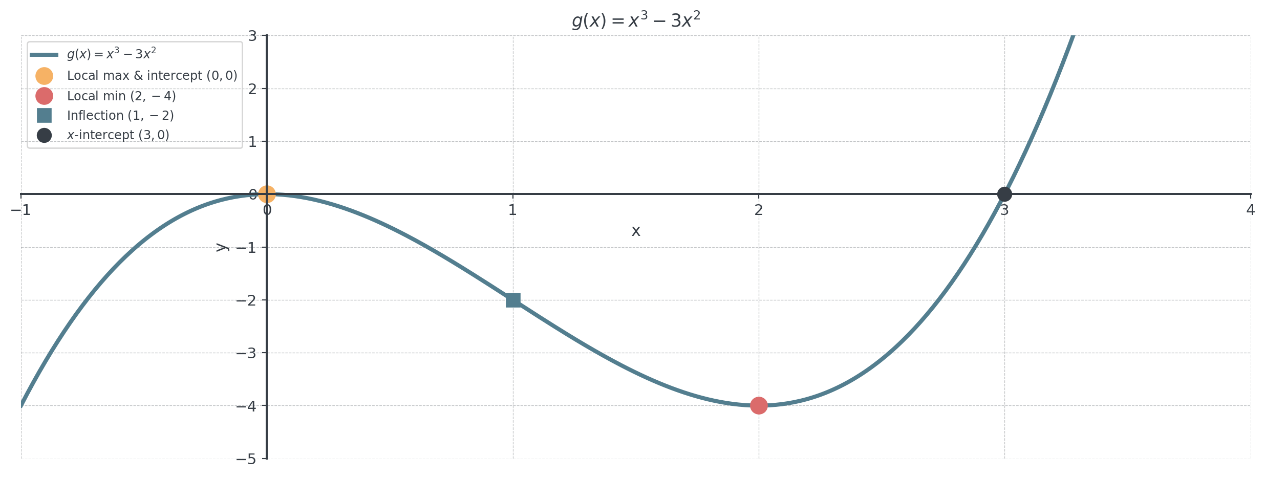
Problem: Sketch \(g(x) = x^3 - 3x^2\)

Step 1: Domain and Intercepts

• Domain: All reals
• \(y\)-intercept: \(g(0) = 0\)
• \(x\)-intercepts: Solve \(x^3 - 3x^2 = x^2(x - 3) = 0 \implies x = 0, \, x = 3\)

Steps 2: Critical Points

Problem: Sketch \(g(x) = x^3 - 3x^2\)

. . .

Classification using first derivative:

. . .

\[g'(x) = 3x^2 - 6x\]

. . .

\[3x(x - 2) = 0\]

. . .

\[x = 0 \text{ or } x = 2\]

. . .

Rather easy, right?

Steps 3: Inflection Points

Problem: Sketch \(g(x) = x^3 - 3x^2\)

. . .

Classification using second derivative:

. . .

\[g''(x) = 6x - 6\]

. . .

• \(g''(0) = -6 < 0\) → local max at \(x = 0\)
• \(g''(2) = 6 > 0\) → local min at \(x = 2\)

. . .

Inflection points:

. . .

\[g''(x) = 6x - 6 = 0 \implies x = 1\]

Steps 4 & 5: Sign Charts and Behavior

Problem: Sketch \(g(x) = x^3 - 3x^2\)

. . .

\(g'(x) = 3x(x-2)\):

. . .

• \((+)\) for \(x < 0\), \((-)\) for \(0 < x < 2\), \((+)\) for \(x > 2\)

. . .

\(g''(x) = 6x - 6 = 6(x-1)\):

. . .

• \((-)\) for \(x < 1\) (concave down), \((+)\) for \(x > 1\) (concave up)

. . .

End behavior:

. . .

• As \(x \to -\infty\): \(g(x) \to -\infty\) (leading term \(x^3\))
• As \(x \to +\infty\): \(g(x) \to +\infty\)

Step 6: Complete Sketch

Guided Practice - 25 Minutes

Set A - Work in Pairs

Complete these problems in pairs

1. Find and classify all critical points of \(f(x) = x^4 - 4x^3 + 10\) using the second derivative test.

2. Find the absolute extrema of \(g(x) = x^3 - 3x^2 + 1\) on \([-1, 3]\).

3. For \(h(x) = \frac{x^2 + 1}{x}\), find: (a) domain, (b) intercepts, (c) asymptotes.

4. Determine the intervals where \(f(x) = x^3 - 3x + 2\) is increasing and decreasing.

Set B - Work in Pairs

Continue with your partner

1. Sketch a sign chart for \(f'(x)\) and \(f''(x)\) where \(f(x) = x^4 - 2x^2\).

2. Find all inflection points of \(g(x) = x^4 - 4x^3 + 6\).

3. For \(h(x) = 2x^3 - 9x^2 + 12x\), find the absolute extrema on \([0, 3]\).

4. Determine the concavity intervals for \(f(x) = x^3 - 6x^2 + 9x\).

Coffee Break - 15 Minutes

Business Applications

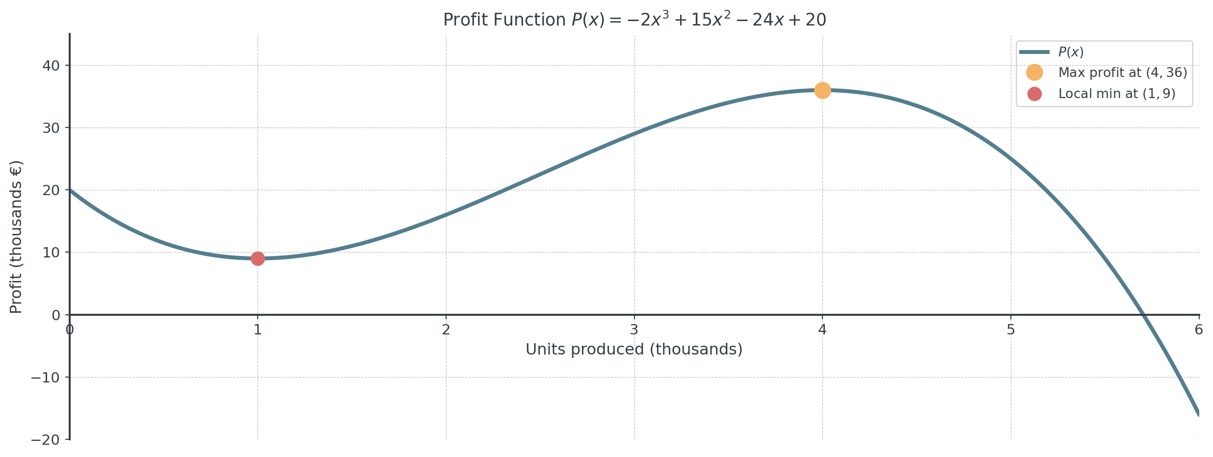
Application 1: Profit Maximization

A company’s profit function (in thousands) is:

\[P(x) = -2x^3 + 15x^2 - 24x + 20\]

where \(x\) is the number of units produced (in thousands).

. . .

Question: Find the production level that maximizes profit.

. . .

1. Find critical points:

. . .

\[P'(x) = -6x^2 + 30x - 24 = -6(x^2 - 5x + 4) = -6(x-1)(x-4)\]

. . .

Critical points: \(x = 1\) and \(x = 4\)

Classification of Critical Points

2. Use second derivative test:

. . .

\[P''(x) = -12x + 30\]

. . .

• At \(x = 1\): \(P''(1) = -12 + 30 = 18 > 0\) → local minimum
• At \(x = 4\): \(P''(4) = -48 + 30 = -18 < 0\) → local maximum
• Answer: Maximum profit occurs at \(x = 4\) (4000 units)

. . .

3. Calculate profit at critical maximum point:

• \(P(4) = -2(64) + 15(16) - 24(4) + 20 = -128 + 240 - 96 + 20 = 36\)
• Maximum profit: €36,000 at 4000 units

Visualizing Profit

. . .

The max on the left is cut off because we have to produce at least 0 units.

Application 2: Cost Minimization

Average cost per unit for a manufacturer is:

\[\bar{C}(x) = \frac{100}{x} + 2x + 5\]

where \(x\) is batch size (in hundreds).

. . .

Question: What batch size minimizes average cost?

Critical Points

1. Find critical points:

\[\bar{C}'(x) = -\frac{100}{x^2} + 2\]

. . .

\[-\frac{100}{x^2} + 2 = 0\]

. . .

\[2 = \frac{100}{x^2}\]

. . .

\[x^2 = 50\]

. . .

\[x = \sqrt{50} = 5\sqrt{2} \approx 7.07\]

Verification and Answer

2. Verify it’s a minimum using second derivative:

• \(\bar{C}''(x) = \frac{200}{x^3}\)
• At \(x = 5\sqrt{2}\): \(\bar{C}''(5\sqrt{2}) = \frac{200}{(5\sqrt{2})^3} > 0\) → minimum

. . .

3. Minimum average cost:

• \(\bar{C}(5\sqrt{2}) = \frac{100}{5\sqrt{2}} + 2(5\sqrt{2}) + 5 = \frac{20}{\sqrt{2}} + 10\sqrt{2} + 5\)
• \(10\sqrt{2} + 10\sqrt{2} + 5 = 20\sqrt{2} + 5 \approx 33.28\)
• Answer: Batch size of 707 units minimizes average cost at approximately €33.28 per unit

Application 3: Revenue Maximization

A company’s revenue function is where \(x\) is units sold (in thousands): \[R(x) = 50x - 0.5x^2\]

. . .

Question: What level maximizes revenue, and what is the maximum?

• \(R'(x) = 50 - x = 0\) → \(x = 50\)
• Verify: \(R''(x) = -1 < 0\) → maximum!
• Maximum: \(R(50) = 50(50) - 0.5(50)^2 = 2500 - 1250 = 1250\)
• Answer: €1,250,000 at 50,000 units sold

Collaborative Problem-Solving - 30 Minutes

Group Challenge I

Scenario: A manufacturing company has the following functions:

• Cost: \(C(x) = 1000 + 5x + 0.01x^2\) (in euros)
• Revenue: \(R(x) = 25x - 0.02x^2\) (in euros)

where \(x\) is the number of units produced and sold.

Group Challenge II

Work in groups of 3-4 students

1. Find the profit function \(P(x) = R(x) - C(x)\).

2. Determine the production level that maximizes profit.

3. What is the maximum profit?

4. Find the break-even points (where \(P(x) = 0\)).

5. Sketch the profit function showing all key features.

6. What production range yields positive profit?

Think-Pair-Share - 7 Minutes

Reflection Question

Think individually (2 min), then discuss with class

• In business optimization, why is it important to check both the first and second derivatives?
• Give a specific example where the second derivative test would reveal critical information about a business decision.

Optimization Checklist

Before finalizing any optimization answer, always verify:

1. Is the critical point actually a maximum (if maximizing) or minimum (if minimizing)?
2. Did you check the second derivative sign?
3. Did you consider endpoint constraints?
4. Does the answer make business sense? (positive quantities, reasonable values)

. . .

Show your verification work! Examiners want to see you confirmed the type of extremum!

Wrap-Up & Key Takeaways

Summary of Session 05-06

Derivative Tests:

• First derivative test: Examine sign changes of \(f'\) to classify
• Second derivative test: Use \(f''(c)\) to classify when \(f'(c) = 0\)
  • \(f''(c) > 0\) → local min; \(f''(c) < 0\) → local max

. . .

Global Extrema:

• On closed interval \([a, b]\): check critical points AND endpoints
• Largest value = absolute max; smallest value = absolute min

Curve Sketching Algorithm Recap

Question: Can anyone summarize the steps to sketching a curve?

. . .

1. Domain & intercepts
2. Critical points
3. Inflection points
4. Sign charts (\(f'\) and \(f''\))
5. Asymptotes & end behavior
6. Complete sketch

. . .

Follow these in the Feststellungsprüfung!

Final Assessment - 5 Minutes

Quick Check

Complete individually - this helps me assess today’s learning

1. For \(f(x) = x^3 - 3x^2\), find all critical points and classify them using the second derivative test.

2. Find the absolute extrema of \(g(x) = x^2 - 4x + 1\) on \([0, 4]\).

3. A profit function is \(P(x) = -x^2 + 100x - 500\). What production level maximizes profit?

4. True or False: If \(f''(c) = 0\), then \(x = c\) is always an inflection point.

Next Session Preview

Looking Ahead: Session 05-07

Function Determination & Related Rates

. . .

What’s coming:

• Finding functions from conditions (points, slopes, extrema)
• Setting up systems of equations from constraints
• Related rates problems (changing quantities)
• The 5-step strategy for related rates
• Business applications: cost functions, demand rates

. . .

Repeat the 6-step curve sketching algorithm! Both function determination and related rates share a key skill: setting up equations from conditions systematically.