Tasks 05-01 - Limits & Continuity Through Graphs
Section 05: Differential Calculus
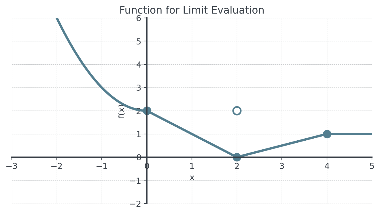
Problem 1: Basic Limit Evaluation (x)
Given the graph below, evaluate the following limits:
Determine \(\lim_{x \to 0} f(x)\)
Compute \(\lim_{x \to 2^-} f(x)\) and \(\lim_{x \to 2^+} f(x)\)
Verify whether \(\lim_{x \to 2} f(x)\) exists. If it does, give its value.
Explain why \(\lim_{x \to 4} f(x) = 1\)
CautionSolution
- Determination of \(\lim_{x \to 0} f(x)\):
- From the left (x < 0): The function is \(f(x) = x^2 + 2\), so as \(x \to 0^-\), we get \(0^2 + 2 = 2\)
- From the right (x > 0): The function is \(f(x) = -x + 2\), so as \(x \to 0^+\), we get \(-0 + 2 = 2\)
- Since both one-sided limits equal 2, \(\lim_{x \to 0} f(x) = 2\)
- Computation of one-sided limits at x = 2:
- Left-hand limit: For \(x < 2\), we use \(f(x) = -x + 2\)
- \(\lim_{x \to 2^-} f(x) = -2 + 2 = 0\)
- Right-hand limit: For \(x > 2\), we use \(f(x) = 0.5x - 1\)
- \(\lim_{x \to 2^+} f(x) = 0.5(2) - 1 = 0\)
- Left-hand limit: For \(x < 2\), we use \(f(x) = -x + 2\)
- Verification of limit existence:
- Since \(\lim_{x \to 2^-} f(x) = 0\) and \(\lim_{x \to 2^+} f(x) = 0\)
- Both one-sided limits are equal
- Therefore, \(\lim_{x \to 2} f(x) = 0\) exists
- Note: The function value \(f(2) = 0\) exists, and the limit equals this value, so the function is continuous at \(x = 2\).
- Explanation for \(\lim_{x \to 4} f(x) = 1\):
- From the left (x < 4): The function is \(f(x) = 0.5x - 1\), so \(\lim_{x \to 4^-} f(x) = 0.5(4) - 1 = 1\)
- From the right (x > 4): The function is \(f(x) = 1\) (constant), so \(\lim_{x \to 4^+} f(x) = 1\)
- Since both one-sided limits equal 1, the limit exists and equals 1
- Additionally, \(f(4) = 1\), so the function is continuous at \(x = 4\)
Problem 2: One-Sided Limits and Discontinuities (x)
A company’s discount policy is given by the following function, where \(D(x)\) represents the discount percentage for an order of \(x\) units:
\[D(x) = \begin{cases} 0 & \text{if } 0 < x < 50 \\ 5 & \text{if } x = 50 \\ 10 & \text{if } 50 < x < 100 \\ 15 & \text{if } x \geq 100 \end{cases}\]
Determine \(\lim_{x \to 50^-} D(x)\) and \(\lim_{x \to 50^+} D(x)\)
Compute \(\lim_{x \to 100^-} D(x)\) and \(\lim_{x \to 100^+} D(x)\)
Verify whether the discount function is continuous at \(x = 50\) and \(x = 100\)
Sketch the graph of \(D(x)\) for \(0 < x < 150\)
CautionSolution
- One-sided limits at x = 50:
- Left-hand limit: For \(x < 50\), \(D(x) = 0\)
- Therefore, \(\lim_{x \to 50^-} D(x) = 0\)
- Right-hand limit: For \(x > 50\), \(D(x) = 10\)
- Therefore, \(\lim_{x \to 50^+} D(x) = 10\)
- Left-hand limit: For \(x < 50\), \(D(x) = 0\)
- One-sided limits at x = 100:
- Left-hand limit: For \(x < 100\), \(D(x) = 10\)
- Therefore, \(\lim_{x \to 100^-} D(x) = 10\)
- Right-hand limit: For \(x \geq 100\), \(D(x) = 15\)
- Therefore, \(\lim_{x \to 100^+} D(x) = 15\)
- Left-hand limit: For \(x < 100\), \(D(x) = 10\)
- Continuity check:
- At x = 50:
- \(D(50) = 5\) (defined)
- \(\lim_{x \to 50^-} D(x) = 0\) and \(\lim_{x \to 50^+} D(x) = 10\)
- Since the one-sided limits are different, the limit doesn’t exist
- Not continuous at x = 50 (jump discontinuity)
- At x = 100:
- \(D(100) = 15\) (defined)
- \(\lim_{x \to 100^-} D(x) = 10\) and \(\lim_{x \to 100^+} D(x) = 15\)
- The one-sided limits are different
- Not continuous at x = 100 (jump discontinuity)
- At x = 50:
- Graph of D(x):
The graph shows the discount policy as a step function with three horizontal segments: 0% for quantities below 50, 10% for quantities between 50 and 100, and 15% for quantities above 100. There are jump discontinuities at x = 50 and x = 100, with open circles at the endpoints of each segment and a filled isolated point at (50, 5).
Interpretation: The discount policy has jump discontinuities at the threshold quantities, which might discourage orders of exactly 50 units (since customers get only 5% instead of 10%).
Problem 3: Tax Bracket Analysis (xx)
A progressive tax system has the following marginal tax rates:
| Income Range | Marginal Tax Rate |
|---|---|
| €0 - €20,000 | 0% |
| €20,001 - €50,000 | 20% |
| €50,001 - €100,000 | 30% |
| Above €100,000 | 40% |
The tax owed function \(T(x)\) for income \(x\) is:
\[T(x) = \begin{cases} 0 & \text{if } 0 \leq x \leq 20000 \\ 0.2(x - 20000) & \text{if } 20000 < x \leq 50000 \\ 6000 + 0.3(x - 50000) & \text{if } 50000 < x \leq 100000 \\ 21000 + 0.4(x - 100000) & \text{if } x > 100000 \end{cases}\]
Investigate the continuity of \(T(x)\) at the bracket boundaries: €20,000, €50,000, and €100,000.
Compute the effective tax rate \(E(x) = \frac{T(x)}{x}\) for incomes of €19,999, €20,001, €49,999, and €50,001.
Argue why it’s important that \(T(x)\) is continuous while the marginal rate function is not.
Graph both \(T(x)\) and the marginal tax rate function for \(0 \leq x \leq 150000\).
CautionSolution
Continuity investigation at boundaries:
At x = €20,000:
- \(T(20000) = 0\) (using first piece)
- \(\lim_{x \to 20000^-} T(x) = 0\)
- \(\lim_{x \to 20000^+} T(x) = 0.2(20000 - 20000) = 0\)
- All three are equal, so continuous at €20,000
At x = €50,000:
- From below: \(\lim_{x \to 50000^-} T(x) = 0.2(50000 - 20000) = 6000\)
- From above: \(\lim_{x \to 50000^+} T(x) = 6000 + 0.3(50000 - 50000) = 6000\)
- \(T(50000) = 0.2(30000) = 6000\)
- All equal, so continuous at €50,000
At x = €100,000:
- From below: \(\lim_{x \to 100000^-} T(x) = 6000 + 0.3(50000) = 21000\)
- From above: \(\lim_{x \to 100000^+} T(x) = 21000 + 0.4(0) = 21000\)
- \(T(100000) = 6000 + 15000 = 21000\)
- All equal, so continuous at €100,000
Effective tax rates:
- €19,999: \(E(19999) = \frac{0}{19999} = 0\%\)
- €20,001: \(E(20001) = \frac{0.2(1)}{20001} = \frac{0.2}{20001} \approx 0.001\%\)
- €49,999: \(E(49999) = \frac{0.2(29999)}{49999} = \frac{5999.8}{49999} \approx 12.0\%\)
- €50,001: \(E(50001) = \frac{6000 + 0.3(1)}{50001} = \frac{6000.3}{50001} \approx 12.0\%\)
Importance of continuity:
- Fairness: A €1 increase in income should never decrease after-tax income
- No cliff effects: Continuous tax prevents situations where earning slightly more results in paying significantly more tax
- Predictability: Small changes in income lead to small changes in tax
- Incentive preservation: No disincentive to earn slightly more
- The marginal rate can jump because it only affects the additional income, not all previous income
Graphs:
Two side-by-side graphs are shown. Left: The tax function T(x) is a continuous piecewise linear curve that starts at 0, remains flat until 20k, then increases with slopes of 0.2, 0.3, and 0.4 in successive brackets. Right: The marginal tax rate is a step function with jumps at the bracket boundaries (20k, 50k, 100k), showing rates of 0%, 20%, 30%, and 40%. Dashed vertical lines mark the bracket transitions.
Observation: The tax owed increases smoothly (continuous) while the marginal rate jumps at boundaries.
Problem 4: Business Application - Production Cost Model (xx)
A manufacturer has different production methods available depending on quantity:
- Hand-crafted (0-50 units): \(C_1(x) = 100x + 200\)
- Semi-automated (50-200 units): \(C_2(x) = 40x + 3200\)
- Fully automated (200+ units): \(C_3(x) = 25x + 6200\)
The actual cost function includes a one-time setup cost of €500 when switching methods.
Determine the complete cost function \(C(x)\) including setup costs at transition points.
Calculate all limits at the transition points \(x = 50\) and \(x = 200\).
Assess whether it’s ever beneficial to produce exactly 50 or 200 units.
Decide on the optimal production quantity if demand is estimated between 180 and 220 units. Substantiate your recommendation.
CautionSolution
Complete cost function with setup costs:
At transition points, we add €500 setup cost:
\[C(x) = \begin{cases} 100x + 200 & \text{if } 0 < x < 50 \\ 100(50) + 200 + 500 & \text{if } x = 50 \\ 40x + 3200 & \text{if } 50 < x < 200 \\ 40(200) + 3200 + 500 & \text{if } x = 200 \\ 25x + 6200 & \text{if } x > 200 \end{cases}\]
Simplifying: \[C(x) = \begin{cases} 100x + 200 & \text{if } 0 < x < 50 \\ 5700 & \text{if } x = 50 \\ 40x + 3200 & \text{if } 50 < x < 200 \\ 11700 & \text{if } x = 200 \\ 25x + 6200 & \text{if } x > 200 \end{cases}\]
Limits at transition points:
At x = 50:
- \(\lim_{x \to 50^-} C(x) = 100(50) + 200 = 5200\)
- \(\lim_{x \to 50^+} C(x) = 40(50) + 3200 = 5200\)
- \(C(50) = 5700\) (includes setup cost)
- Limit exists and equals €5200, but function is discontinuous
At x = 200:
- \(\lim_{x \to 200^-} C(x) = 40(200) + 3200 = 11200\)
- \(\lim_{x \to 200^+} C(x) = 25(200) + 6200 = 11200\)
- \(C(200) = 11700\) (includes setup cost)
- Limit exists and equals €11200, but function is discontinuous
Analysis of producing exactly at transition points:
- At x = 50:
- Cost = €5700 (with setup)
- Cost at 49 units: €5100
- Cost at 51 units: €5240
- Never beneficial to produce exactly 50 units
- At x = 200:
- Cost = €11700 (with setup)
- Cost at 199 units: €11160
- Cost at 201 units: €11225
- Never beneficial to produce exactly 200 units
The €500 setup cost creates a “penalty” for producing at transition quantities.
- At x = 50:
Optimal production for 180-220 unit demand:
Let’s analyze costs in this range:
Quantity Method Cost Calculation Total Cost 180 Semi-automated 40(180) + 3200 €10,400 190 Semi-automated 40(190) + 3200 €10,800 199 Semi-automated 40(199) + 3200 €11,160 200 Transition Special case €11,700 201 Fully automated 25(201) + 6200 €11,225 210 Fully automated 25(210) + 6200 €11,450 220 Fully automated 25(220) + 6200 €11,700 The graph shows total cost in the 180-220 unit range. The semi-automated line (slope 40) rises from left until x = 200, where there is a jump discontinuity: an open circle at (200, 11200) and a filled circle at (200, 11700) representing the setup cost spike. Beyond 200, the fully automated line continues with a lower slope of 25.
Recommendation:
- If demand ≤ 199 units: Use semi-automated production
- If demand ≥ 201 units: Use fully automated production
- Avoid exactly 200 units due to setup cost penalty
- The break-even point (ignoring setup) is where: \(40x + 3200 = 25x + 6200\) \(15x = 3000\) \(x = 200\) units
Since the methods have equal cost at 200 units (without setup), and the fully automated method has lower marginal cost (€25 vs €40), choose fully automated for any quantity above 200 units.
Problem 5: Rational Function Analysis (xxx)
Consider the rational function: \[f(x) = \frac{x^3 - 8}{x^2 - 4}\]
Show that this function can be simplified and identify any holes.
Investigate the behavior of \(f(x)\) as \(x\) approaches 2 and -2. Determine all relevant limits.
Verify whether \(f\) can be made continuous by redefining it at certain points. If so, give the continuous extension.
Sketch the complete graph of \(f\), clearly marking all discontinuities, asymptotes, and key features.
Interpret this function as a cost model where discontinuities represent equipment failures. Explain the economic implications.
CautionSolution
Simplification and holes:
Factor numerator and denominator:
- Numerator: \(x^3 - 8 = (x - 2)(x^2 + 2x + 4)\)
- Denominator: \(x^2 - 4 = (x - 2)(x + 2)\)
Therefore: \[f(x) = \frac{(x - 2)(x^2 + 2x + 4)}{(x - 2)(x + 2)}\]
For \(x \neq 2\): \[f(x) = \frac{x^2 + 2x + 4}{x + 2}\]
Hole at x = 2 (removable discontinuity) Vertical asymptote at x = -2 (non-removable)
Behavior analysis:
As x → 2: Using the simplified form:
- \(\lim_{x \to 2} f(x) = \lim_{x \to 2} \frac{x^2 + 2x + 4}{x + 2} = \frac{4 + 4 + 4}{4} = 3\)
- Both one-sided limits equal 3
- But \(f(2)\) is undefined (hole)
As x → -2:
- From the left: \(\lim_{x \to -2^-} f(x) = -\infty\) (denominator → 0⁻, numerator → 4)
- From the right: \(\lim_{x \to -2^+} f(x) = +\infty\) (denominator → 0⁺, numerator → 4)
- Vertical asymptote at x = -2
Continuous extension:
Define the continuous extension: \[g(x) = \begin{cases} \frac{x^3 - 8}{x^2 - 4} & \text{if } x \neq 2, -2 \\ 3 & \text{if } x = 2 \end{cases}\]
This makes the function continuous at x = 2. The discontinuity at x = -2 cannot be removed (infinite discontinuity).
Complete graph:
The graph shows the rational function with three separate branches. There is a vertical asymptote at x = -2 (dashed line), where the function approaches negative infinity from the left and positive infinity from the right. A removable discontinuity (hole) is marked with an open circle at (2, 3). The y-intercept is at (0, 2). A dashed oblique asymptote y = x shows the long-run behavior of the function.
Key features:
- Hole at (2, 3) - removable discontinuity
- Vertical asymptote at x = -2
- Oblique asymptote: y = x (found by polynomial division)
- y-intercept: (0, 2)
- No x-intercepts (numerator never equals zero after cancellation)
Economic interpretation as cost model:
Let \(f(x)\) represent average cost per unit when producing \(x + 2\) thousand units (shifting to avoid negative production).
- Hole at x = 2 (4000 units): Temporary equipment malfunction
- Production briefly impossible at exactly this level
- Can be “patched” by maintenance (continuous extension)
- Nearby production levels unaffected
- Vertical asymptote at x = -2 (0 units): Fundamental limitation
- Costs approach infinity as production approaches zero
- Fixed costs dominate at very low production
- Cannot be remedied - structural issue
- Oblique asymptote y = x: Long-run behavior
- Average costs grow linearly at high production
- Diseconomies of scale emerge
- Capacity constraints binding
Business implications:
- Plan to avoid exactly 4000 units (or have contingency)
- Never attempt near-zero production
- Consider splitting large orders to avoid diseconomies
- Hole at x = 2 (4000 units): Temporary equipment malfunction
Problem 6: Complex Production Optimization (xxx)
A tech company manufactures smart home devices with a complex cost structure that depends on production volume and quality level. The cost function is:
\[C(x, q) = \begin{cases} 1000 + 50x + 10qx & \text{if } 0 < x < 100 \text{ (Prototype phase)} \\ 5000 + 30x + 8qx & \text{if } 100 \leq x < 500 \text{ (Small batch)} \\ 8000 + 25x + 5qx & \text{if } x \geq 500 \text{ (Mass production)} \end{cases}\]
where \(x\) is the number of units and \(q\) is the quality level (1 ≤ q ≤ 5).
The revenue function is \(R(x, q) = x \cdot (80 + 20q)\) (higher quality commands higher prices).
Part A: Continuity Analysis
Investigate whether the cost function is continuous at the transition points x = 100 and x = 500 for a fixed quality level q = 3.
Determine all quality levels \(q\) for which the cost function is continuous at x = 100.
Part B: Profit Optimization
Calculate the profit function \(P(x, q) = R(x, q) - C(x, q)\) for each production phase when q = 3.
Decide which production level maximizes profit if the company can produce between 450 and 550 units. Consider the transition at x = 500.
Graph the profit function for q = 3 over the range 0 < x < 700 and mark all discontinuities.
Argue whether the company should implement a continuous cost structure. What are the trade-offs?
CautionSolution
Part A: Continuity Analysis
Continuity check at transition points for q = 3:
At x = 100:
- From prototype phase: \(\lim_{x \to 100^-} C(x, 3) = 1000 + 50(100) + 10(3)(100) = 1000 + 5000 + 3000 = 9000\)
- From small batch: \(\lim_{x \to 100^+} C(x, 3) = 5000 + 30(100) + 8(3)(100) = 5000 + 3000 + 2400 = 10400\)
- \(C(100, 3) = 10400\) (uses small batch formula since 100 ∈ [100, 500))
- Not continuous - jump of €1400
At x = 500:
- From small batch: \(\lim_{x \to 500^-} C(x, 3) = 5000 + 30(500) + 8(3)(500) = 5000 + 15000 + 12000 = 32000\)
- From mass production: \(\lim_{x \to 500^+} C(x, 3) = 8000 + 25(500) + 5(3)(500) = 8000 + 12500 + 7500 = 28000\)
- \(C(500, 3) = 28000\) (uses mass production formula)
- Not continuous - jump of €4000 (costs actually decrease!)
Finding q for continuity at x = 100:
For continuity, we need: \(1000 + 50(100) + 10q(100) = 5000 + 30(100) + 8q(100)\) \(1000 + 5000 + 1000q = 5000 + 3000 + 800q\) \(6000 + 1000q = 8000 + 800q\) \(200q = 2000\) \(q = 10\)
Since q must be between 1 and 5, no quality level makes the cost continuous at x = 100.
Part B: Profit Optimization
Profit function for q = 3:
Revenue: \(R(x, 3) = x(80 + 20(3)) = 140x\)
Profit by phase:
Prototype (0 < x < 100): \(P(x, 3) = 140x - (1000 + 50x + 30x) = 60x - 1000\)
Small batch (100 ≤ x < 500): \(P(x, 3) = 140x - (5000 + 30x + 24x) = 86x - 5000\)
Mass production (x ≥ 500): \(P(x, 3) = 140x - (8000 + 25x + 15x) = 100x - 8000\)
Optimal production for 450-550 units:
Evaluate profit at key points:
- P(450, 3) = 86(450) - 5000 = 38700 - 5000 = €33,700
- P(499, 3) = 86(499) - 5000 = 42914 - 5000 = €37,914
- P(500, 3) = 100(500) - 8000 = 50000 - 8000 = €42,000
- P(501, 3) = 100(501) - 8000 = 50100 - 8000 = €42,100
- P(550, 3) = 100(550) - 8000 = 55000 - 8000 = €47,000
Recommendation: Produce 550 units (maximum in range) for €47,000 profit.
The jump to mass production at x = 500 creates a significant profit increase despite higher fixed costs.
Profit function graph:
The graph shows the profit function for q=3 across three production phases. The prototype phase (slope 60) transitions to the small batch phase (slope 86) at x = 100, where profit drops by approximately 1400 euros. The small batch phase transitions to mass production (slope 100) at x = 500, where profit jumps up by approximately 4086 euros. A horizontal dashed line marks zero profit, with break-even points labeled at approximately x = 17, x = 58, and x = 80.
- Analysis of continuous vs. discontinuous cost structure:
Arguments for continuous structure:
- Predictability: Smooth cost changes make planning easier
- No perverse incentives: Avoids situations where producing less costs more per unit
- Customer relations: Can offer consistent pricing
- Operational stability: No sudden jumps in resource needs
Arguments for keeping discontinuous structure:
- Reflects reality: Setup costs and equipment changes are real
- Economies of scale: Large batches genuinely reduce per-unit costs
- Investment clarity: Clear thresholds for equipment upgrades
- Competitive advantage: Mass production efficiency rewards scale
Trade-offs:
- Short-term flexibility vs. long-term efficiency
- Smooth operations vs. cost optimization
- Risk management vs. profit maximization
Recommendation: Keep the discontinuous structure but: 1. Plan production to avoid being just below thresholds 2. Communicate clearly with customers about volume pricing 3. Consider volume commitments to reach efficient scale 4. Use the jumps as strategic decision points for capacity expansion
The €4,086 profit jump at x=500 represents real economies of scale that shouldn’t be smoothed away artificially.