Session 06-04 - Area Between Curves & Economic Surplus

Section 06: Integral Calculus

Author

Dr. Nikolai Heinrichs & Dr. Tobias Vlcek

Entry Quiz - 10 Minutes

Quick Review from Session 06-03

Test your understanding of Area Problems

Find the total area between \(f(x) = x - 2\) and the x-axis from \(x = 0\) to \(x = 4\).
Evaluate \(\int_0^2 3e^{2x} \, dx\)
Evaluate \(\int_1^e \frac{4}{x} \, dx\)
If a production rate is \(P(t) = 100 - 5t\), find total production from \(t = 0\) to \(t = 10\).

Homework Discussion - 15 Minutes

Your questions from Session 06-03

Focus on area problems and special integrals

Handling regions above and below the x-axis
Exponential and logarithmic integrals
Business applications of area
Setting up integrals from word problems

. . .

Today we find the area between two curves and apply this to economic surplus!

Learning Objectives

What You’ll Master Today

Find intersection points of two functions algebraically
Determine which function is on top in each region
Set up integrals for area between curves: \(\int_a^b [f(x) - g(x)] \, dx\)
Handle multiple regions when curves cross
Calculate Consumer and Producer Surplus using areas
Find equilibrium and interpret market efficiency

. . .

Area between curves is the foundation for understanding economic surplus!

Part A: The Basic Concept

Area Between Two Curves

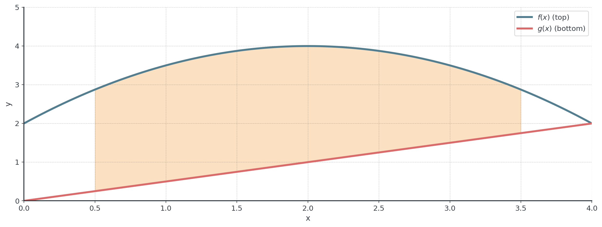
Key idea: If \(f(x) \geq g(x)\) on \([a, b]\), then: \(\text{Area} = \int_a^b [f(x) - g(x)] \, dx\)

. . .

Top curve minus bottom curve!

Why Does This Work?

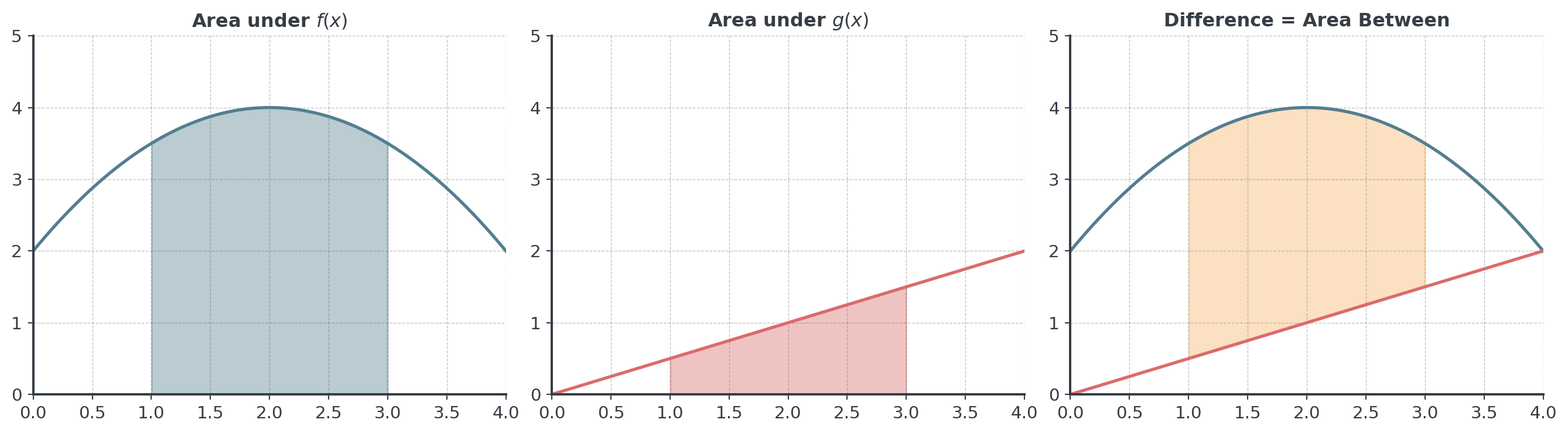
Think of it as subtracting areas:

. . .

\[\int_a^b f(x) \, dx - \int_a^b g(x) \, dx = \int_a^b [f(x) - g(x)] \, dx\]

The Formula

Area between curves:

. . .

\[\text{Area} = \int_a^b |f(x) - g(x)| \, dx\]

Or if you know \(f(x) \geq g(x)\):

\[\text{Area} = \int_a^b [f(x) - g(x)] \, dx\]

. . .

Find intersection points (bounds \(a\) and \(b\)), determine which function is on top and then integrate top minus bottom.

Part B: Finding Intersection Points

Setting Up the Problem

To find where curves intersect:

. . .

Set \(f(x) = g(x)\) and solve for \(x\).

. . .

Example: Find where \(f(x) = 6 - x^2\) and \(g(x) = x\) intersect.

. . .

\[6 - x^2 = x\] \[x^2 + x - 6 = 0\] \[(x + 3)(x - 2) = 0\] \[x = -3 \text{ or } x = 2\]

Example: Complete Solution

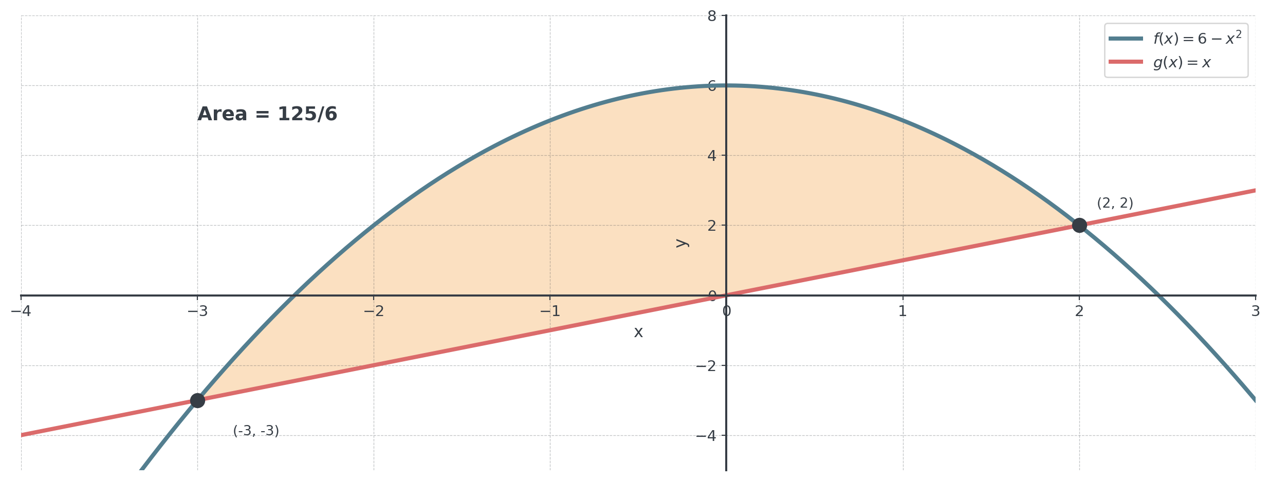
Find the area between \(f(x) = 6 - x^2\) and \(g(x) = x\).

Step 1: Intersection points are \(x = -3\) and \(x = 2\) ✓
Step 2: Which is on top? Test \(x = 0\):
- \(f(0) = 6\)
- \(g(0) = 0\)
- So \(f(x) \geq g(x)\) on \([-3, 2]\) ✓
Step 3: Calculate the area:
- \(\int_{-3}^{2} [(6 - x^2) - x] \, dx = \int_{-3}^{2} (6 - x - x^2) \, dx\)

Completing the Calculation

\[\int_{-3}^{2} (6 - x - x^2) \, dx = \left[6x - \frac{x^2}{2} - \frac{x^3}{3}\right]_{-3}^{2}\]

. . .

At \(x = 2\): \(12 - 2 - \frac{8}{3} = 10 - \frac{8}{3} = \frac{22}{3}\)

. . .

At \(x = -3\): \(-18 - \frac{9}{2} + 9 = -9 - \frac{9}{2} = -\frac{27}{2}\)

. . .

\[\text{Area} = \frac{22}{3} - \left(-\frac{27}{2}\right) = \frac{22}{3} + \frac{27}{2} = \frac{44 + 81}{6} = \frac{125}{6}\]

Visualization

. . .

Even though part of this region lies below the x-axis, the area is still positive because we integrate \((f(x) - g(x))\) where \(f\) is above \(g\).

Break - 10 Minutes

Part C: When Curves Cross

Strategy for Crossing Curves

When curves cross:

Find all intersection points
Split the interval at each crossing
In each region, determine which curve is on top
Calculate area of each region separately
Add all regions (all positive)

. . .

\[\text{Total Area} = \int_{a}^{c} |f - g| \, dx + \int_{c}^{b} |f - g| \, dx\]

Example: Crossing Curves

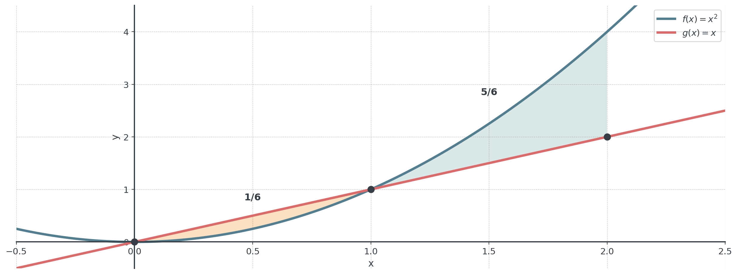
Find the area between \(f(x) = x^2\) and \(g(x) = x\) from \(x = 0\) to \(x = 2\).

Step 1: Find intersections on \([0, 2]\):
- \(x^2 = x \implies x^2 - x = 0 \implies x(x-1) = 0\)
- Intersections at \(x = 0\) and \(x = 1\)
Step 2: Determine which is on top:
- On \([0, 1]\): Test \(x = 0.5\): \(f(0.5) = 0.25\), \(g(0.5) = 0.5\). So \(g > f\)
- On \([1, 2]\): Test \(x = 1.5\): \(f(1.5) = 2.25\), \(g(1.5) = 1.5\). So \(f > g\)
Step 3: Calculate each region (next slide)

Calculate each Region

Region 1 \((0 \leq x \leq 1)\): \(g\) on top

. . .

\[\int_0^1 (x - x^2) \, dx = \left[\frac{x^2}{2} - \frac{x^3}{3}\right]_0^1 = \frac{1}{2} - \frac{1}{3} = \frac{1}{6}\]

. . .

Region 2 \((1 \leq x \leq 2)\): \(f\) on top

. . .

\[\int_1^2 (x^2 - x) \, dx = \left[\frac{x^3}{3} - \frac{x^2}{2}\right]_1^2 = \left(\frac{8}{3} - 2\right) - \left(\frac{1}{3} - \frac{1}{2}\right) = \frac{2}{3} + \frac{1}{6} = \frac{5}{6}\]

. . .

Total Area \(= \frac{1}{6} + \frac{5}{6} = 1\)

Visualization

. . .

Total Area = 1/6 + 5/6 = 1

Guided Practice - 20 Minutes

Set A: Basic Area Between Curves

Work individually for 8 minutes

Find the area between \(f(x) = x^2\) and \(g(x) = 4\) from \(x = -2\) to \(x = 2\).
Find the area between \(f(x) = x + 2\) and \(g(x) = x^2\) (find intersection points first).
Find the area between \(y = \sqrt{x}\) and \(y = x\) for \(x \in [0, 1]\).

Practice Set B: Curves That Cross

Work individually for 6 minutes

Find the area enclosed between \(f(x) = 4 - x^2\) and \(g(x) = 3x\) from \(x = -1\) to \(x = 1\).
Find the total area between \(f(x) = x^3\) and \(g(x) = x\) from \(x = -1\) to \(x = 1\).

Coffee Break - 15 Minutes

Part D: Consumer Surplus

The Economic Intuition

Consumers benefit when they pay less than their willingness to pay

. . .

Example: If you’d pay up to 80 EUR for a concert ticket but it costs 50 EUR…

Your consumer surplus = 80 - 50 = 30 EUR
This is the “bonus” you receive from the transaction

. . .

For an entire market, we sum up all individual surpluses using integration!

Consumer Surplus Formula

Definition: Area between demand curve and equilibrium, from 0 to \(q^*\):

. . .

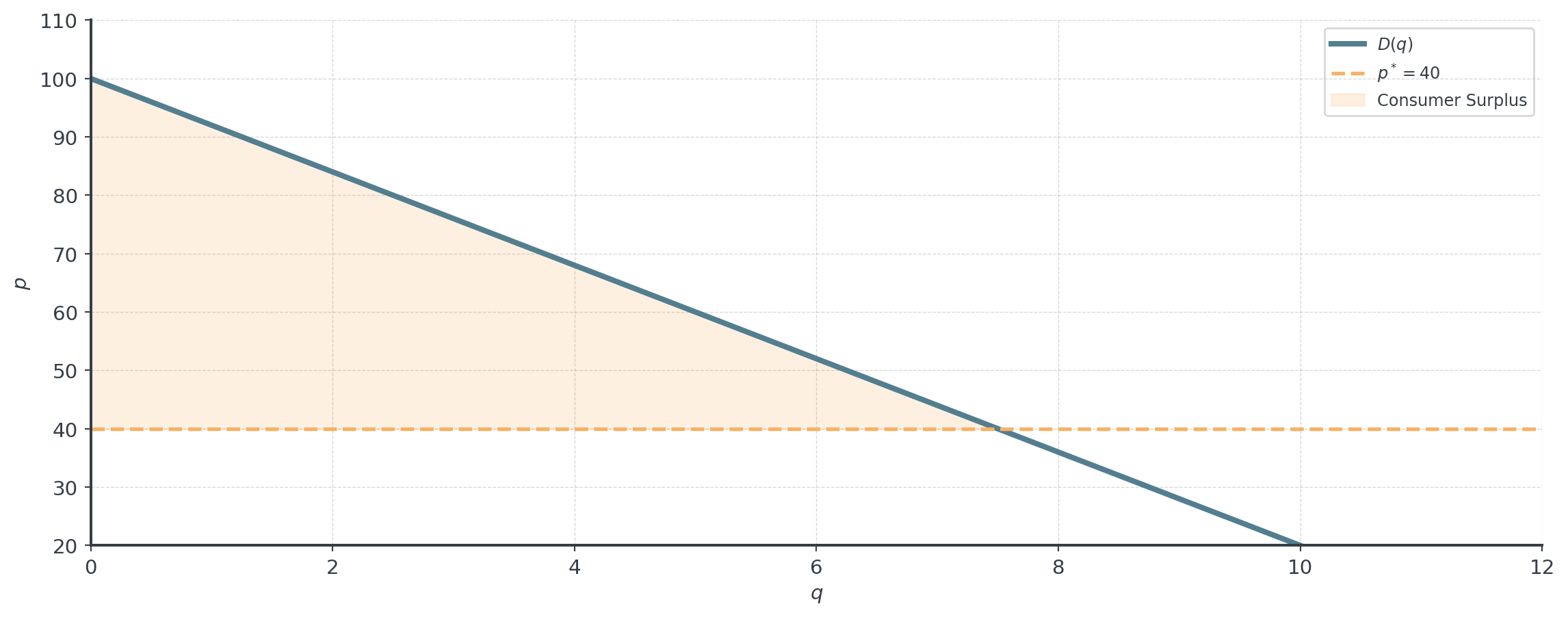
\(CS = \int_0^{q^*} [D(q) - p^*] \, dq\)

Example: Computing Surplus

Demand curve: \(D(q) = 100 - 4q\) EUR, equilibrium at \(q^* = 15\) units, \(p^* = 40\) EUR

. . .

\[CS = \int_0^{15} [(100 - 4q) - 40] \, dq\]

. . .

\[= \int_0^{15} (60 - 4q) \, dq\]

. . .

\[= \left[60q - 2q^2\right]_0^{15}\]

. . .

\[= 900 - 450 = 450 \text{ EUR}\]

Part E: Producer Surplus

The Economic Intuition

Producers benefit when they receive more than their minimum acceptable price

. . .

Example: If a farmer would sell wheat for minimum 30 EUR/unit but receives 50 EUR…

Their producer surplus = 50 - 30 = 20 EUR per unit
This is their “bonus” from the transaction

. . .

For an entire market, we sum up all producer surpluses using integration!

Producer Surplus Formula

Definition: Area between equilibrium and supply curve, from 0 to \(q^*\):

. . .

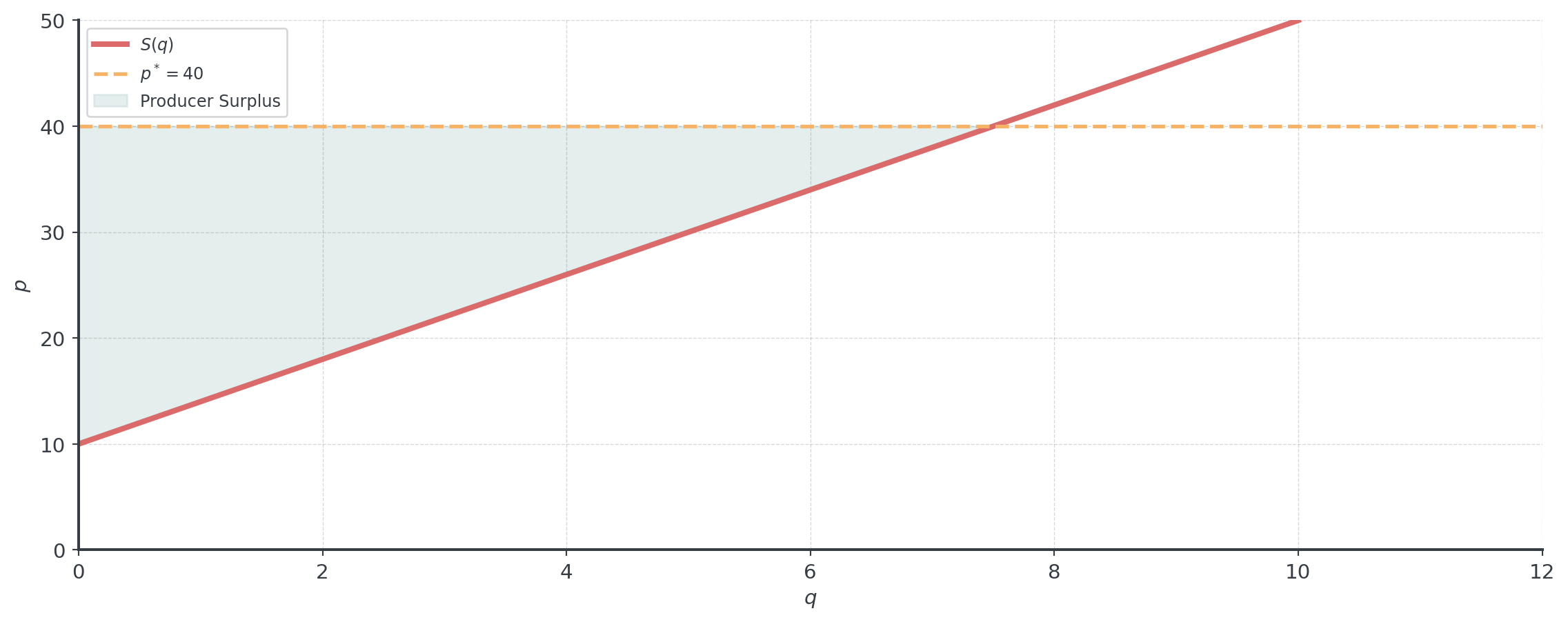
\(PS = \int_0^{q^*} [p^* - S(q)] \, dq\)

Example: Computing Producer Surplus

Supply curve: \(S(q) = 10 + 2q\) EUR, equilibrium at \(q^* = 15\) units, \(p^* = 40\) EUR

. . .

\[PS = \int_0^{15} [40 - (10 + 2q)] \, dq\]

. . .

\[= \int_0^{15} (30 - 2q) \, dq\]

. . .

\[= \left[30q - q^2\right]_0^{15}\]

. . .

\[= 450 - 225 = 225 \text{ EUR}\]

Part F: Market Equilibrium & Total Surplus

Finding Equilibrium

At equilibrium: Demand equals Supply, so \(D(q) = S(q)\)

. . .

Example: \(D(q) = 120 - 3q\) and \(S(q) = 20 + q\)

. . .

\[120 - 3q = 20 + q\] \[100 = 4q\] \[q^* = 25\]

. . .

\[p^* = 120 - 3(25) = 45 \text{ EUR}\]

. . .

Always verify: \(S(25) = 20 + 25 = 45\) ✓

Total Surplus

Total Surplus = Consumer Surplus + Producer Surplus

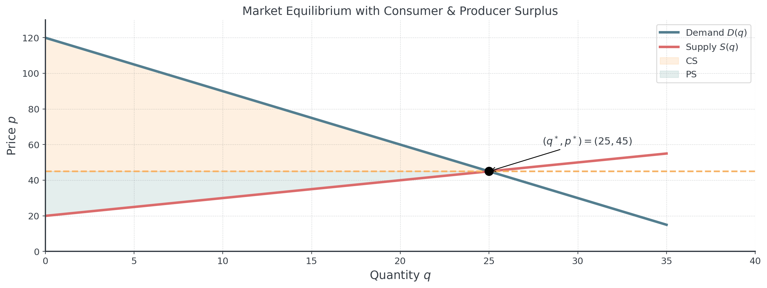
Complete Market Analysis I

Given: \(D(q) = 120 - 3q\), \(S(q) = 20 + q\), equilibrium \((q^*, p^*) = (25, 45)\)

. . .

Consumer Surplus: \[CS = \int_0^{25} [(120 - 3q) - 45] \, dq = \int_0^{25} (75 - 3q) \, dq\]

. . .

\[= \left[75q - \frac{3q^2}{2}\right]_0^{25} = 1875 - 937.5 = 937.5 \text{ EUR}\]

Complete Market Analysis II

Producer Surplus: \[PS = \int_0^{25} [45 - (20 + q)] \, dq = \int_0^{25} (25 - q) \, dq\]

. . .

\[= \left[25q - \frac{q^2}{2}\right]_0^{25} = 625 - 312.5 = 312.5 \text{ EUR}\]

. . .

Total Surplus: \(937.5 + 312.5 = 1250\) EUR

Total surplus measures the total economic benefit a market generates for all participants. It equals the area between the demand and supply curves up to the equilibrium quantity. At equilibrium, total surplus is maximized. Any deviation, e.g., through price controls or taxes, would reduce it.

Collaborative Problem-Solving - 30 Minutes

Set C: Market Analysis

Work in pairs for 10 minutes

A market has demand \(D(q) = 150 - 5q\) and supply \(S(q) = 30 + 3q\).

Find equilibrium \((q^*, p^*)\)
Calculate CS and PS
Find total surplus

Market Analysis with Price Floor

Scenario: A regional for organic produce has (\(q\) is quantity in tons):

Demand: \(D(q) = 80 - 0.5q\) (price in EUR)
Supply: \(S(q) = 20 + 0.25q\) (price in EUR)

Find the equilibrium quantity and price.
Calculate consumer surplus and producer surplus at equilibrium.
If a price floor of EUR 50 is imposed:
- What quantity is demanded? What quantity is supplied?
- Calculate the new CS and PS (up to quantity traded).
Compare the surpluses. Sketch both scenarios on the same graph.

Wrap-Up & Key Takeaways

Today’s Essential Concepts

Area between curves: \(\int_a^b [f(x) - g(x)] \, dx\) where \(f \geq g\)
Finding bounds: Set \(f(x) = g(x)\) to find intersection points
Multiple regions: Split at crossings, sum absolute values
Consumer Surplus: \(CS = \int_0^{q^*} [D(q) - p^*] \, dq\)
Producer Surplus: \(PS = \int_0^{q^*} [p^* - S(q)] \, dq\)
Total Surplus: CS + PS = total benefit to society

. . .

Next session: Integration by Parts and Synthesis!

Final Assessment - 5 Minutes

Quick Check

Work individually, then compare

Find the area between \(f(x) = 4 - x\) and \(g(x) = x\) from \(x = 0\) to \(x = 2\).
If demand is \(D(q) = 100 - 2q\) and supply is \(S(q) = 20 + q\), find equilibrium \((q^*, p^*)\).
For the market in problem 2, set up (but don’t evaluate) the integrals for CS and PS.

Next Session Preview

Coming Up: Integration by Parts

Integration by Parts: The reverse product rule
LIATE Rule: How to choose \(u\) and \(dv\)
Common integrals: \(\int x e^x \, dx\), \(\int x \ln x \, dx\)
Average Value of a function
Revenue and Cost accumulation over time
Synthesis: Combining optimization and integration

. . .

Complete Tasks 06-04

Practice finding intersection points
Work on area between curves problems