Session 06-02 - Definite Integrals & The Fundamental Theorem

Section 06: Integral Calculus

Author

Dr. Nikolai Heinrichs & Dr. Tobias Vlćek

Entry Quiz - 10 Minutes

Quick Review from Session 06-01

Test your understanding of Antiderivatives

Find \(\int (4x^3 - 6x + 2) \, dx\)
Find \(\int \frac{3}{x^2} \, dx\)
If \(f'(x) = 2x + 1\) and \(f(0) = 3\), find \(f(x)\).
Why do we write \(+C\) when finding indefinite integrals?

Homework Discussion - 15 Minutes

Your questions from Session 06-01

Focus on antiderivatives and indefinite integrals

Challenges with the power rule
Initial value problems
Business applications (marginal cost → total cost)
Verification by differentiation

. . .

Today we connect integration to area and discover the Fundamental Theorem of Calculus!

Learning Objectives

What You’ll Master Today

Understand the definite integral as a limit of sums
Interpret definite integrals as signed area under curves
Apply the Fundamental Theorem of Calculus to evaluate integrals
Use the evaluation formula \(\int_a^b f(x) \, dx = F(b) - F(a)\)
Apply properties of definite integrals
Interpret net change using definite integrals
Connect integration to accumulation in business contexts

. . .

The Fundamental Theorem connects the area problem to antiderivatives!

Part A: The Area Problem

Motivating Question

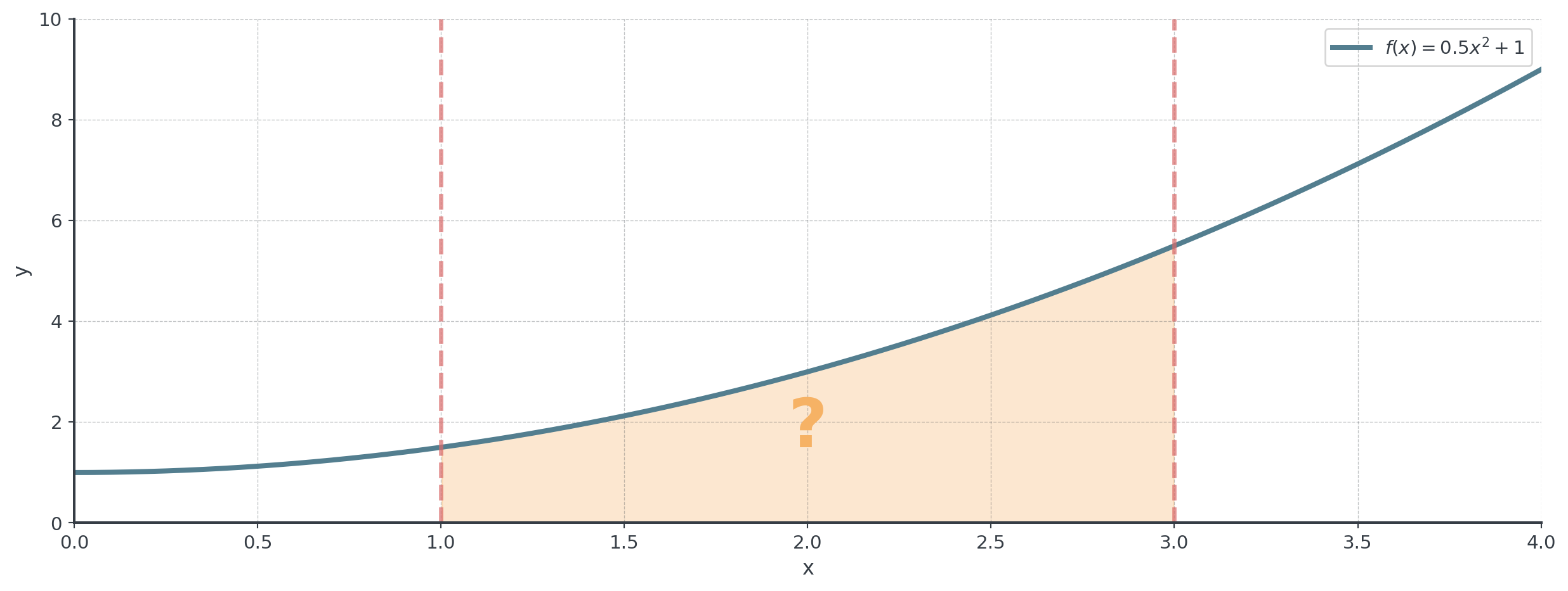
How do we find the area under a curve?

. . .

Question: What is the area of the shaded region between \(x = 1\) and \(x = 3\)?

The Rectangle Approximation Idea

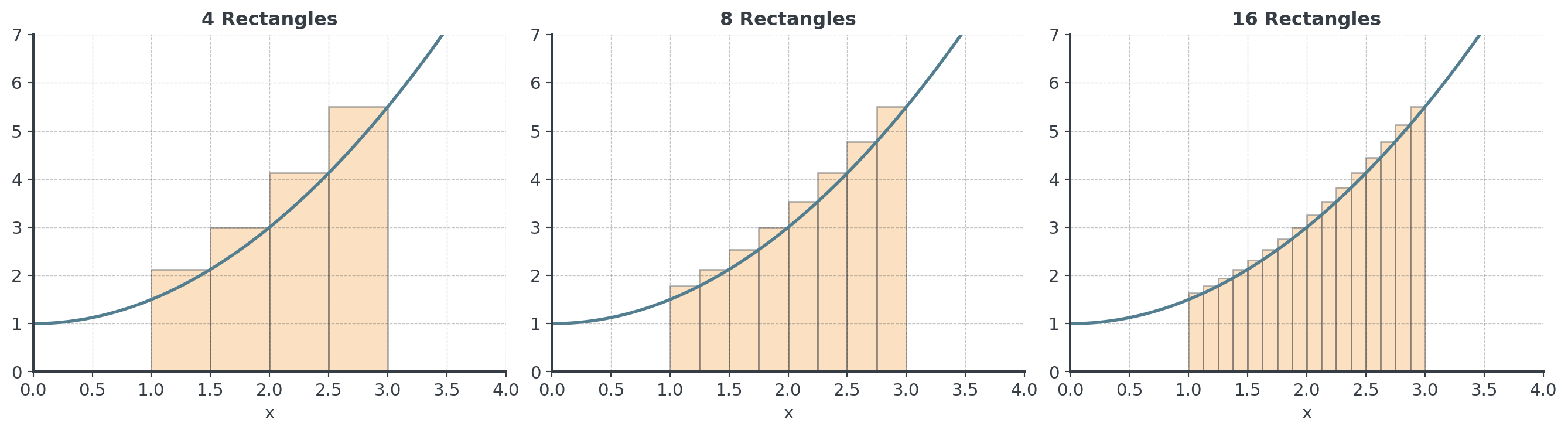
Strategy: Approximate the curved region with rectangles!

. . .

More rectangles → Better approximation!

The Riemann Sum

Definition: A Riemann sum approximates area using rectangles:

\[\sum_{i=1}^{n} f(x_i^*) \cdot \Delta x\]

. . .

\(\Delta x = \frac{b-a}{n}\) is the width of each rectangle
\(x_i^*\) is a sample point in the \(i\)-th subinterval
\(f(x_i^*)\) is the height of the \(i\)-th rectangle
We sum the areas of all \(n\) rectangles
As \(n \to \infty\), the Riemann sum approaches the exact area!

From Sum to Integral

The Definite Integral:

\[\int_a^b f(x) \, dx = \lim_{n \to \infty} \sum_{i=1}^{n} f(x_i^*) \cdot \Delta x\]

\(\int_a^b\) means “integrate from \(a\) to \(b\)”
\(a\) is the lower limit of integration
\(b\) is the upper limit of integration
The result is a number (not a function!)

Part B: Signed Area

Area Above vs. Below the x-axis

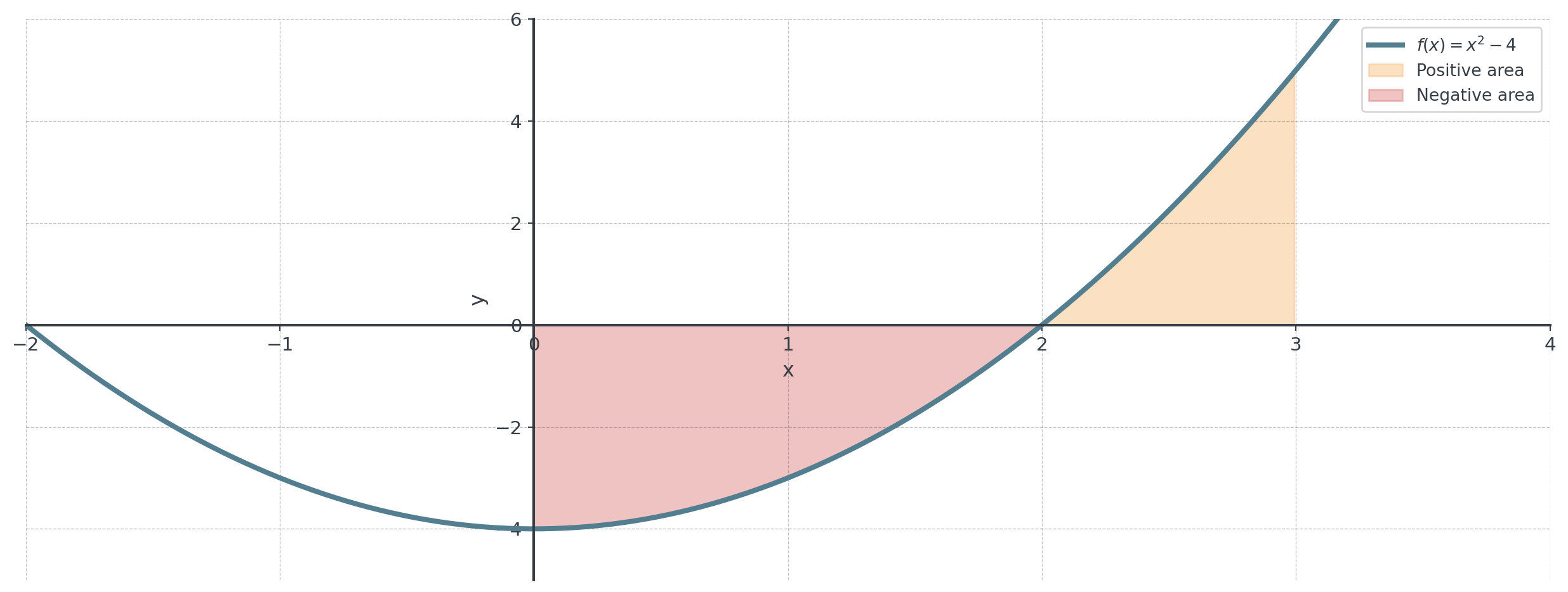
Key insight: Definite integrals measure signed area!

Signed Area Rules

The definite integral gives signed area:

Above x-axis: Area counts as positive
Below x-axis: Area counts as negative
Total: Positive area minus negative area

. . .

Signed area ≠ Total area

If you want total (unsigned) area, you need to handle regions above and below separately!

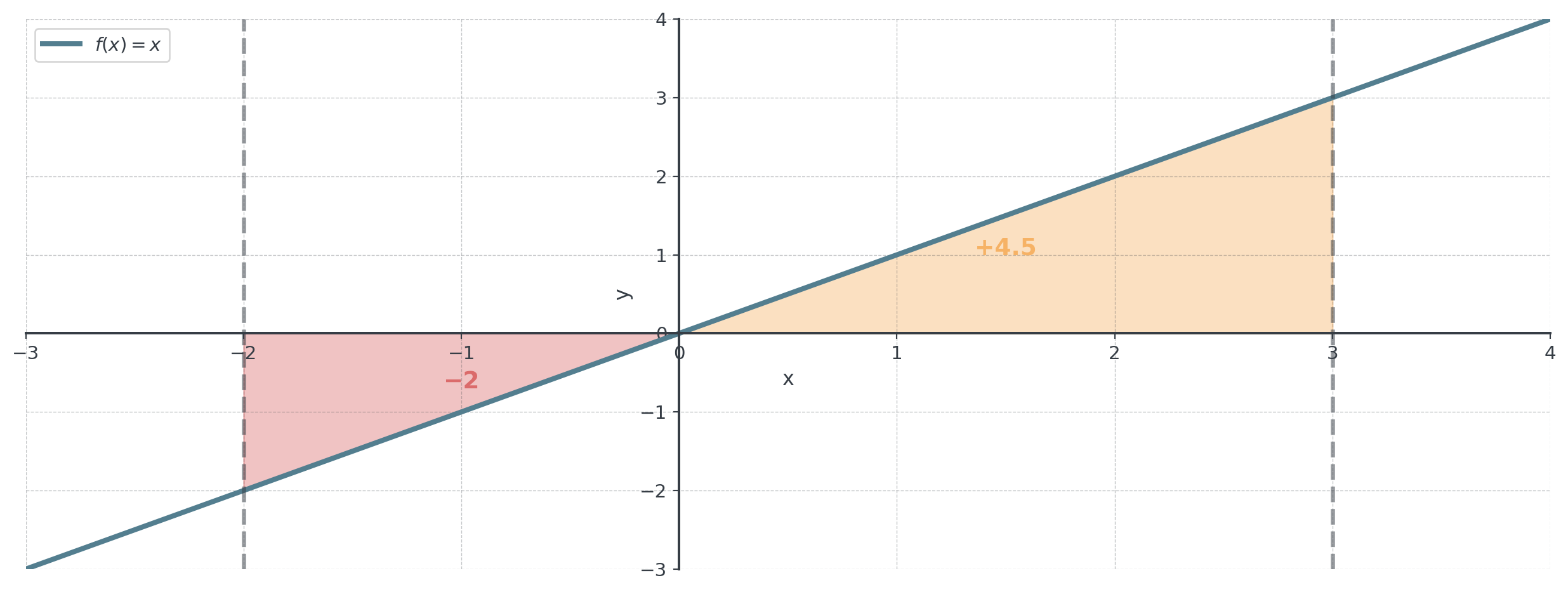
Example: Signed vs. Total Area

. . .

Signed area: \(\int_{-2}^{3} x \, dx = 4.5 - 2 = 2.5\)
Total area: \(|{-2}| + 4.5 = 6.5\)

Break - 10 Minutes

Part C: The Fundamental Theorem of Calculus

The Big Connection

The Fundamental Theorem of Calculus (FTC):

. . .

If \(F(x)\) is an antiderivative of \(f(x)\), then:

\[\int_a^b f(x) \, dx = F(b) - F(a)\]

. . .

This is one of the most important theorems in mathematics! It connects:

Differentiation (finding rates of change)
Integration (finding accumulated quantities/areas)

Why the FTC Works

Intuition: The integral accumulates the rate of change.

\(f(x)\) represents a rate of change
\(F(x)\) represents the total accumulated quantity
\(F(b) - F(a)\) = total change from \(x = a\) to \(x = b\)

. . .

Imagine filling a water tank where \(f(x)\) is the flow rate (liters per minute).

\(F(x)\) is the water level at time \(x\)
So \(F(b) - F(a)\) = (final level) − (initial level) = total liters added!
Each tiny change \(f(x) \cdot \Delta x\) adds up to \(F(b) - F(a)\).

Notation: The Evaluation Bar

We write:

\[\int_a^b f(x) \, dx = F(x) \Big|_a^b = F(b) - F(a)\]

. . .

The notation \(F(x) \Big|_a^b\) means “evaluate \(F\) at \(b\) and subtract \(F\) at \(a\)”

. . .

Also written as:

\[\left[ F(x) \right]_a^b = F(b) - F(a)\]

Example 1: Basic Evaluation

Evaluate: \(\int_1^4 2x \, dx\)

. . .

Step 1: Find an antiderivative

\[F(x) = x^2\]

. . .

Step 2: Apply the FTC

\[\int_1^4 2x \, dx = x^2 \Big|_1^4 = 4^2 - 1^2 = 16 - 1 = 15\]

. . .

No \(+C\) needed for definite integrals! The constants cancel: \((F(b) + C) - (F(a) + C) = F(b) - F(a)\)

Example 2: Polynomial

Evaluate: \(\int_0^3 (x^2 - 2x + 1) \, dx\)

. . .

Step 1: Find an antiderivative

. . .

\[F(x) = \frac{x^3}{3} - x^2 + x\]

. . .

Step 2: Evaluate at bounds

. . .

\[= \left[\frac{x^3}{3} - x^2 + x\right]_0^3 = \left(\frac{27}{3} - 9 + 3\right) - \left(0 - 0 + 0\right)\]

. . .

\[= 9 - 9 + 3 = 3\]

Example 3: With Negative Values

Evaluate: \(\int_{-1}^{2} 3x^2 \, dx\)

. . .

Step 1: Antiderivative is \(F(x) = x^3\)

. . .

Step 2: Evaluate

\[\int_{-1}^{2} 3x^2 \, dx = x^3 \Big|_{-1}^{2} = 2^3 - (-1)^3 = 8 - (-1) = 9\]

. . .

Be careful with negative lower limits! \((-1)^3 = -1\), not \(1\).

Part D: Properties of Definite Integrals

Key Properties

Property 1: Reversing Limits

\[\int_a^b f(x) \, dx = -\int_b^a f(x) \, dx\]

. . .

Property 2: Splitting Intervals

\[\int_a^b f(x) \, dx + \int_b^c f(x) \, dx = \int_a^c f(x) \, dx\]

More Properties

Property 3: Constant Multiple

\[\int_a^b k \cdot f(x) \, dx = k \int_a^b f(x) \, dx\]

. . .

Property 4: Sum/Difference

\[\int_a^b [f(x) \pm g(x)] \, dx = \int_a^b f(x) \, dx \pm \int_a^b g(x) \, dx\]

. . .

These properties are the same as for indefinite integrals, just applied to definite integrals!

Using Properties: Example

Given: \(\int_0^5 f(x) \, dx = 12\) and \(\int_0^3 f(x) \, dx = 7\), find: \(\int_3^5 f(x) \, dx\)

. . .

Solution: Using the splitting property:

\[\int_0^3 f(x) \, dx + \int_3^5 f(x) \, dx = \int_0^5 f(x) \, dx\]

. . .

\[7 + \int_3^5 f(x) \, dx = 12\]

. . .

\[\int_3^5 f(x) \, dx = 5\]

Guided Practice - 20 Minutes

Practice Set A: Basic Evaluation

Work individually for 5 minutes

Evaluate these definite integrals:

\(\int_0^2 3x^2 \, dx\)
\(\int_1^4 (2x - 1) \, dx\)
\(\int_{-2}^{1} x^3 \, dx\)
\(\int_0^1 (x^2 + x + 1) \, dx\)

Practice Set B: More Complex

Work individually for 7 minutes

\(\int_1^9 \frac{2}{\sqrt{x}} \, dx\)
\(\int_{-1}^{3} (4 - x^2) \, dx\)
Given \(\int_0^6 g(x) \, dx = 15\) and \(\int_4^6 g(x) \, dx = 8\), find \(\int_0^4 g(x) \, dx\)
\(\int_2^5 (3x^2 - 4x + 2) \, dx\)

Practice Set C: Area Interpretation

Work in pairs for 8 minutes

Calculate the signed area: \(\int_{-2}^{2} x^3 \, dx\). Explain why this result makes geometric sense.
For \(f(x) = x - 1\) from \(x = 0\) to \(x = 3\):
1. Calculate the signed area \(\int_0^3 (x-1) \, dx\)
2. Find the total (unsigned) area between the curve and x-axis

Coffee Break - 15 Minutes

Part E: The Net Change Theorem

Net Change Interpretation

The Fundamental Theorem as Net Change:

\[\int_a^b f'(x) \, dx = f(b) - f(a)\]

. . .

In words: The integral of a rate of change gives the net change in the original quantity.

. . .

Rate (Derivative)	Integral Gives
Marginal cost \(C'(x)\)	Change in cost \(C(b) - C(a)\)
Population growth rate	Change in population
Production rate	Total production

Business Example: Total Cost Change

Scenario: A company’s marginal cost is \(MC(x) = C'(x) = 20 + 0.5x\) euros per unit. What is the total cost of increasing production from 10 to 50 units?

. . .

Solution:

\[\int_{10}^{50} (20 + 0.5x) \, dx = \left[20x + 0.25x^2\right]_{10}^{50}\]

. . .

\[= (1000 + 625) - (200 + 25) = 1625 - 225 = €1400\]

. . .

The total additional cost of producing 40 more units is €1,400.

Business Example: Monthly Profit Rate

Scenario: A startup’s monthly profit rate (in thousands of euros) is:

\[P'(t) = t^2 - 4t + 3 \text{ (thousands €/month)}\]

where \(t\) is months since launch.

. . .

Question: What is the net profit over the first 4 months?

. . .

Solution:

\[\int_0^4 (t^2 - 4t + 3) \, dt = \left[\frac{t^3}{3} - 2t^2 + 3t\right]_0^4 = \frac{4}{3} \text{ thousand} = €1,333\]

Net Profit vs. Total Cash Flow

Net profit = \(\int_a^b P'(t) \, dt\) (profits minus losses)
Total cash movement = \(\int_a^b |P'(t)| \, dt\) (all money that moved)

. . .

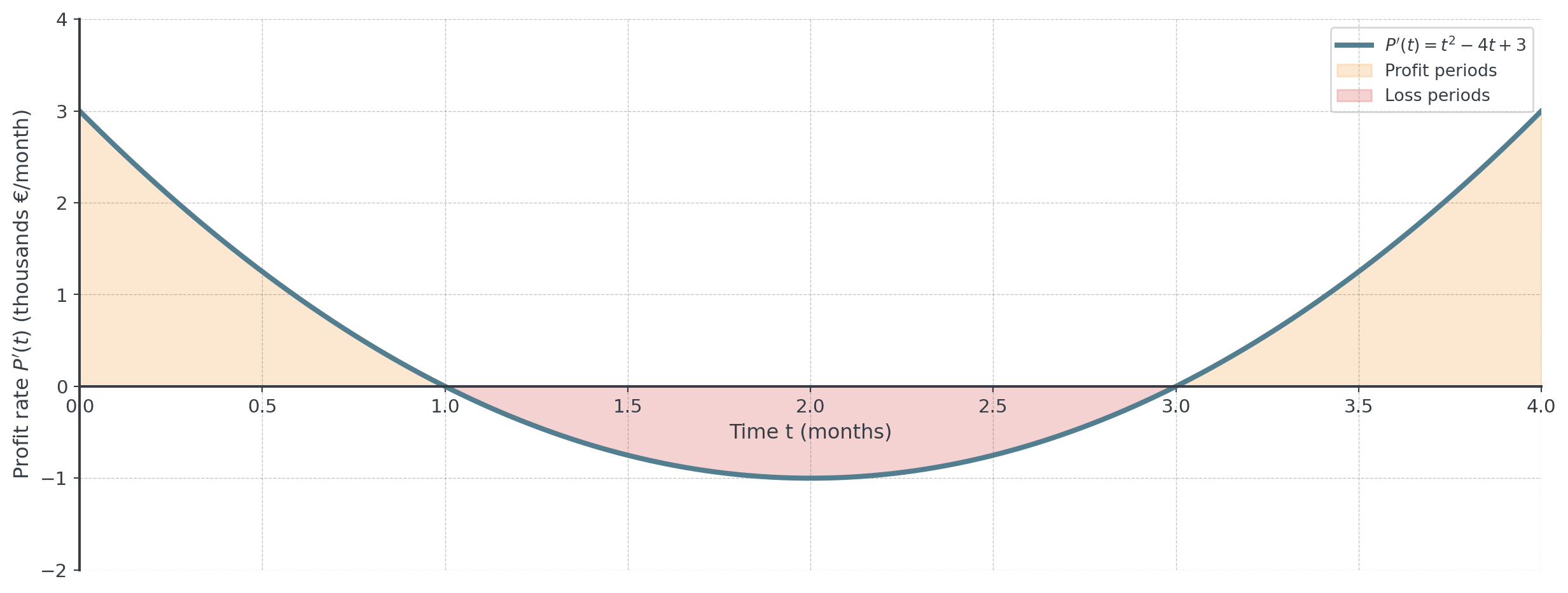
Why Both Measures Matter

Business interpretation:

Months 0-1: Profitable (early adopters)
Months 1-3: Losses (scaling costs exceed revenue)
Months 3-4: Profitable again (economies of scale kick in)

. . .

For investors: Net profit of €1,333 sounds good!

. . .

For cash management: The company needed reserves to survive the loss period (months 1-3), even though it ended up profitable overall.

Collaborative Problem-Solving - 30 Minutes

Group Challenge: Production Analysis

Scenario: A manufacturing plant’s production rate varies during an 8-hour shift:

\[P(t) = 50 + 30t - 3t^2 \text{ units per hour}\]

where \(t\) is hours since the shift started.

Group Tasks

Work in groups of 3-4

Graph \(P(t)\) for \(0 \leq t \leq 8\). At what time is production rate highest?
Calculate the total production during the first 4 hours: \(\int_0^4 P(t) \, dt\)
Calculate total production for the entire 8-hour shift.
When does production rate drop to zero? What does this mean?
If workers are paid €0.50 per unit, calculate total labor cost for:
1. The first half of the shift (0-4 hours)
2. The second half (4-8 hours)

Wrap-Up & Key Takeaways

Today’s Essential Concepts

Definite integral = limit of Riemann sums = signed area
Fundamental Theorem: \(\int_a^b f(x) \, dx = F(b) - F(a)\)
Signed area: Above x-axis positive, below negative
Properties: Reversing limits, splitting intervals, linearity
Net change: \(\int_a^b f'(x) \, dx = f(b) - f(a)\)
Applications: Total cost, displacement, accumulated quantities

. . .

Next session: Area under curves and between curves with applications!

Comparison: Indefinite vs. Definite

Indefinite Integral	Definite Integral
\(\int f(x) \, dx\)	\(\int_a^b f(x) \, dx\)
Result is a function + C	Result is a number
Family of antiderivatives	Signed area / net change
Need \(+C\)	No \(+C\) needed

Final Assessment - 5 Minutes

Quick Check

Work individually, then compare

Evaluate \(\int_1^3 (2x + 4) \, dx\)
If \(\int_0^5 f(x) \, dx = 20\) and \(\int_0^2 f(x) \, dx = 6\), find \(\int_2^5 f(x) \, dx\)
A company’s marginal profit is \(MP(x) = 100 - 2x\). Find the total profit gained by increasing production from 20 to 40 units.

Next Session Preview

Up: Area Problems & Applications

Area under a single curve
Area between a curve and the x-axis
Handling regions where \(f(x) < 0\)
Exponential and logarithmic integrals
Business applications: total profit, accumulated production

. . .

Complete Tasks 06-02

Practice evaluating definite integrals
Focus on the FTC and its applications
Work on signed vs. total area problems