Session 04-03 - Exponential Functions Deep Dive
Section 04: Advanced Functions
Entry Quiz - 10 Minutes
Review from Session 04-02
Work individually for 5 minutes, then we discuss
Simplify: \(\sqrt[3]{8x^6}\)
What is the domain of \(f(x) = \sqrt{x - 4}\)?
Compare the growth rates: Which grows faster for large \(x\): \(x^3\) or \(x^{3.1}\)?
Homework Discussion - 15 Minutes
Your questions from Tasks 04-02
Focus on power functions and economic applications
- Challenges with fractional and negative exponents
- Domain determination strategies
- Growth rate comparison problems
. . .
Exponential functions will show dramatically different growth behavior!
Learning Objectives
Today’s Goals
By the end of this session, you will be able to:
- Understand exponential functions and their unique properties
- Distinguish between exponential growth and decay
- Work with the natural exponential function \(e^x\)
- Apply compound interest formulas in finance
- Model real-world growth and decay processes
- Compare exponential vs. polynomial growth rates
Introduction to Exponential Functions
From Powers to Exponentials
A fundamental shift in perspective
Power Functions: \(f(x) = x^n\) → variable base, fixed exponent
Exponential Functions: \(f(x) = a^x\) → fixed base, variable exponent
. . .
Power: \(x^2\)
- Input: \(2\) → Output: \(4\)
- Input: \(3\) → Output: \(9\)
- Input: \(4\) → Output: \(16\)
Exponential: \(2^x\)
- Input: \(2\) → Output: \(4\)
- Input: \(3\) → Output: \(8\)
- Input: \(4\) → Output: \(16\)
. . .
Key Difference: Exponentials grow MUCH faster than any polynomial!
Definition and Properties
The exponential function family
An exponential function has the form: \[f(x) = a \cdot b^x\]
- \(a \neq 0\) is the initial value (vertical stretch/reflection)
- \(b > 0, b \neq 1\) is the base
. . .
Essential Properties:
- Domain: All real numbers, Range: \((0, \infty)\) when \(a > 0\)
- Always passes through \((0, a)\) and has an inverse
Graphical Behavior
Growth vs. Decay patterns
Exponential Growth Models
The Natural Base e
The most important number in continuous growth
The number \(e ≈ 2.71828...\) is called Euler’s number
- Arises naturally in countless real-world processes
- Foundation for calculus and differential equations
- Base of the natural exponential function \(f(x) = e^x\)
. . .
\[e = \lim_{n \to \infty} \left(1 + \frac{1}{n}\right)^n\]
Properties of \(e^x\)
What makes e special
The function \(f(x) = e^x\) has unique mathematical properties:
- Self-similarity: Rate of change equals value (derivative equals itself)
- Series representation: \(e^x = 1 + x + \frac{x^2}{2!} + \frac{x^3}{3!} + ...\)
- Natural growth: Models any continuous growth or decay process
- Perfect inverse: Has as inverse function the natural logarithm
. . .
Whenever you see continuous processes in nature, business, or science, \(e\) appears!
Visualizing \(e^x\)
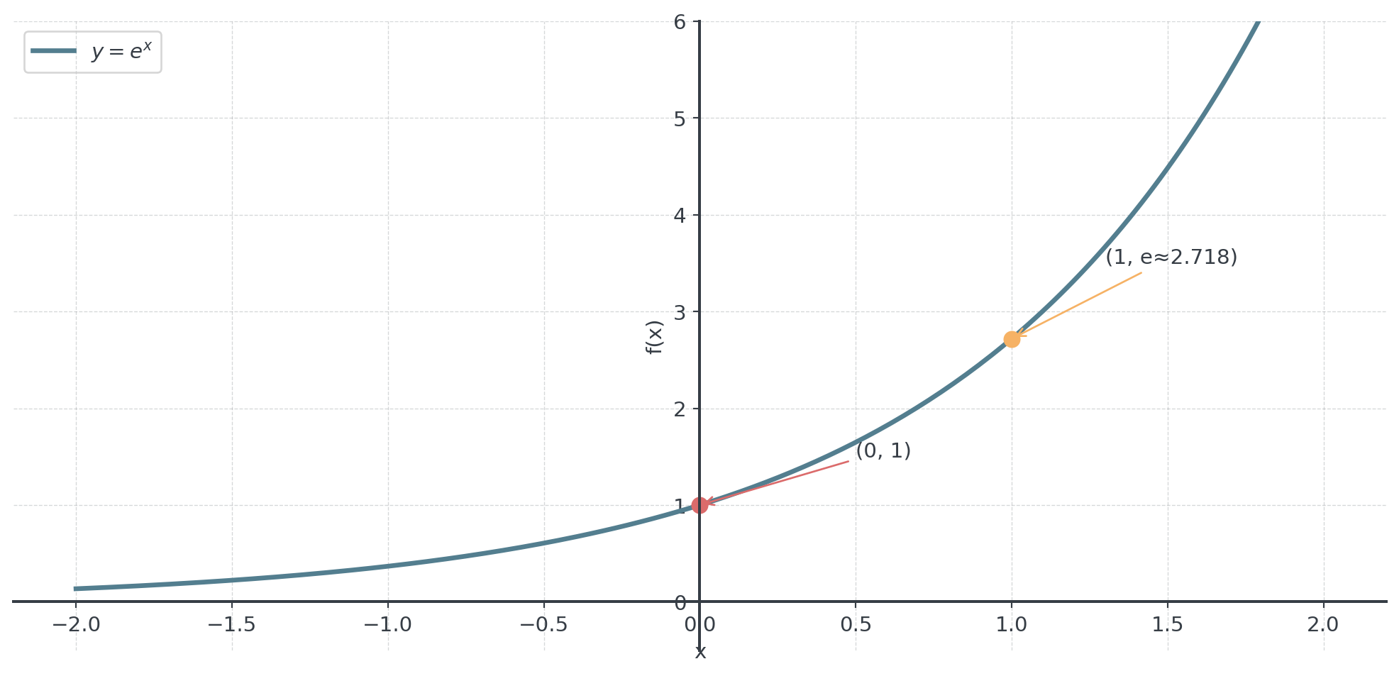
. . .
Always positive, passes through \((0, 1)\), grows faster as \(x\) increases
General Growth Formula
Two equivalent ways to model growth
The general exponential growth model can be written as:
Discrete form: \(A(t) = A_0 \cdot b^t\) where \(b > 1\)
Continuous form: \(A(t) = A_0 \cdot e^{kt}\) where \(k > 0\)
. . .
- \(A_0\) = initial amount
- \(b\) = growth factor (how much it multiplies per period)
- \(k\) = continuous growth rate
- \(t\) = time
. . .
These forms are equivalent! Relationship: \(b = e^k\) or \(k = \ln(b)\)
Business Application: Market Growth
User adoption example
A new app has 1,000 users and grows by 30% monthly.
Discrete model: \(U(t) = 1000 \cdot 1.3^t\) where \(t\) is months
Continuous model: \(U(t) = 1000 \cdot e^{0.2624t}\) (since \(\ln(1.3) ≈ 0.2624\))
. . .
Calculations:
- After 6 months: \(U(6) = 1000 \cdot 1.3^6 ≈ 4,826\) users
- After 12 months: \(U(12) = 1000 \cdot 1.3^{12} ≈ 23,298\) users
. . .
Question: Why might the continuous form be more realistic here?
Break - 10 Minutes
Exponential Decay Models
Decay Processes
When things decrease exponentially
The exponential decay model:
\(A(t) = A_0 \cdot b^t\) where \(0 < b < 1\)
or: \(A(t) = A_0 \cdot e^{-kt}\) where \(k > 0\)
. . .
Question: Any idea where we find this in the real world?
. . .
- Radioactive decay
- Drug concentration in body
- Depreciation of assets
- Cooling processes
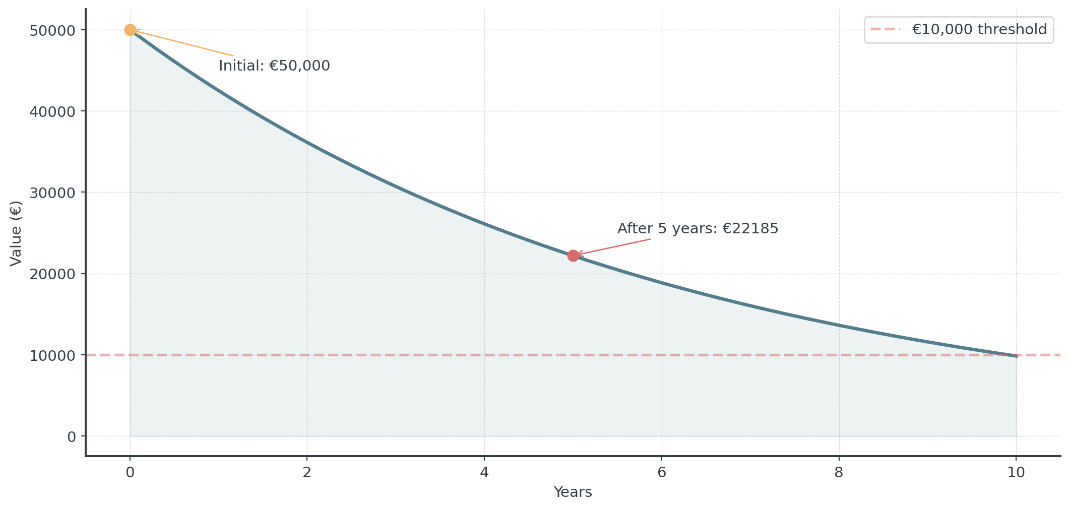
Business Example: Depreciation
A machine costs €50,000 and depreciates 15% annually.
Model: \(V(t) = 50000 \cdot 0.85^t\)
Compound Interest
From Simple to Compound Interest
The power of reinvesting earnings
Simple interest: Only the principal earns interest \[A = P(1 + rt)\]
. . .
Compound interest: Interest earns interest \[A = P\left(1 + \frac{r}{n}\right)^{nt}\]
. . .
- \(P\) = principal (initial investment), \(r\) = annual interest rate
- \(n\) = compounding frequency per year, \(t\) = time in years
Compounding Frequencies
How often interest is calculated matters
Example: €1,000 at 6% annual rate for 1 year
| Frequency | \(n\) value | Formula | Final Amount |
|---|---|---|---|
| Annually | \(n=1\) | \(1000(1.06)^1\) | €1,060.00 |
| Semi-annually | \(n=2\) | \(1000(1.03)^2\) | €1,060.90 |
| Quarterly | \(n=4\) | \(1000(1.015)^4\) | €1,061.36 |
| Monthly | \(n=12\) | \(1000(1.005)^{12}\) | €1,061.68 |
| Daily | \(n=365\) | \(1000(1 + \frac{0.06}{365})^{365}\) | €1,061.83 |
. . .
More frequent compounding → higher returns, but diminishing gains!
Discovering e Through Compounding
Let’s compound €1 at 100% interest for 1 year (\(P=1, r=1, t=1\)):
\[A = \left(1 + \frac{1}{n}\right)^n\]
. . .
- Annually: \((1 + 1)^1 = 2.000\)
- Semi: \((1 + 0.5)^2 = 2.250\)
- Quarterly: \((1 + 0.25)^4 = 2.441\)
- Monthly: \((1.0833...)^{12} = 2.613\)
- Daily: \((1.00274...)^{365} = 2.7146\)
- Hourly: \(≈ 2.7181\)
- Every second: \(≈ 2.71827\)
- As \(n \to \infty\): \(e ≈ 2.71828...\)
. . .
This limit gives us Euler’s number \(e\), the foundation of continuous growth!
Continuous Compounding
The mathematical limit of frequent compounding
As compounding becomes instantaneous (\(n \to \infty\)): \[A = P \cdot e^{rt}\]
. . .
When to use continuous compounding:
- Theoretical maximum return calculations
- Natural growth processes (populations, investments, …)
- Simplifies mathematical analysis
. . .
In practice, continuous vs. daily compounding differs by less than 0.01% for typical rates!
Effective Annual Rate (EAR)
Comparing different compounding methods
The Effective Annual Rate converts any compounding frequency to an equivalent annual rate:
\[\text{EAR} = \left(1 + \frac{r}{n}\right)^n - 1 \quad \text{OR} \quad \text{EAR} = e^r - 1\]
. . .
Example: 6% nominal rate with different compounding
- Monthly: \(\text{EAR} = (1.005)^{12} - 1 = 6.17\%\)
- Continuous: \(\text{EAR} = e^{0.06} - 1 = 6.18\%\)
. . .
Use EAR to compare different investment options fairly!
Spot the Error
Can you identify the errors? Work with your neighbor
Time allocation: 5 minutes to find errors, 5 minutes to discuss
Student work:
“Since \(2^3 = 8\), then \(2^{3x} = 8x\)”
“The function \(f(x) = -2^x\) represents exponential decay”
“If inflation is 3% annually, prices double in \(\frac{100}{3} ≈ 33\) years”
“\((e^2)^3 = e^5\)”
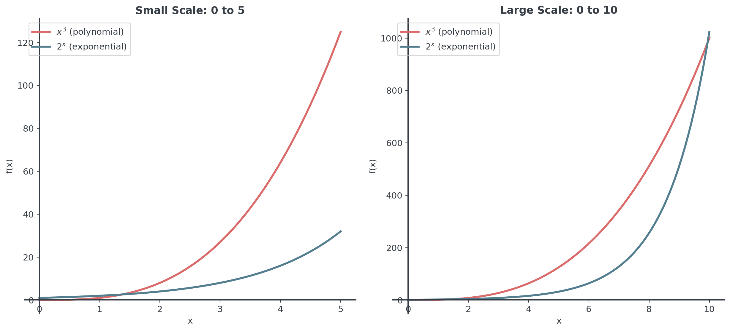
Comparing Growth Rates
Exponential vs. Polynomial
Which wins in the long run?
Comparing Different Bases
How base affects growth rate
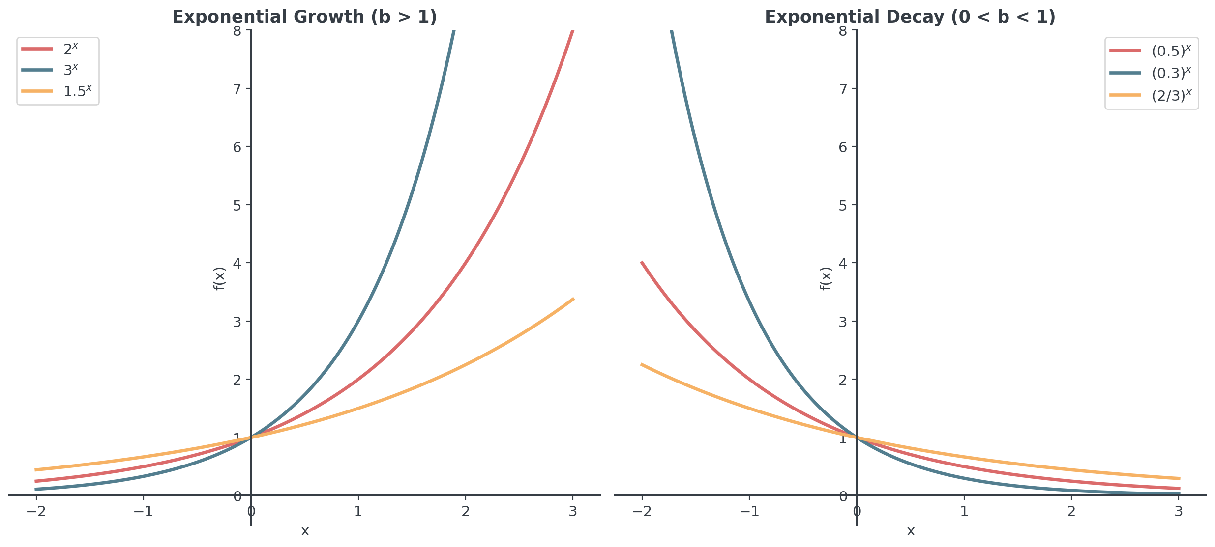
For exponential growth (\(b > 1\)):
- Larger base → faster growth
- \(e^x\) grows faster than \(2^x\) but slower than \(3^x\)
. . .
For exponential decay (\(0 < b < 1\)):
- Smaller base → faster decay
- \((0.3)^x\) decays faster than \((0.5)^x\)
. . .
Remember: The base determines the rate of growth/decay!
Guided Practice - 25 Minutes
Individual Exercise Block I
Work alone for 5 minutes, then discuss for 5 minutes
Problem 1: Population Growth
A bacteria colony starts with 100 cells and triples every 4 hours.
- Write the exponential model \(N(t)\) where \(t\) is hours
- How many bacteria after 12 hours?
- How many bacteria after 16 hours?
- When will the population reach 100,000 cells? (Express as an equation!)
Individual Exercise Block II
Work alone for 5 minutes, then discuss for 5 minutes
Problem 2: Investment Comparison
You have €5,000 to invest for 8 years. Compare:
- Option A: 6% annual rate compounded quarterly
- Option B: 5.9% annual rate compounded continuously
- Calculate the final amount for each option
- Which option is better and by how much?
- What would the continuous rate need to be to match Option A?
Individual Exercise Block III
Work alone for 5 minutes, then discuss for 5 minutes
Problem 3: Half-Life & Medication
A medication has a half-life of 6 hours. You take 200mg.
- Write the decay model \(A(t)\) where \(t\) is hours
- How much remains after 12 hours?
- How much remains after 24 hours?
- After how many half-lives will less than 10mg remain?
Coffee Break - 15 Minutes
Quick Challenge Question
An investment grows from €1,000 to €1,500 in 5 years.
. . .
Question: What was the annual growth rate if compounded continuously?
Real-World Applications
COVID-19 Spread Model
Early pandemic growth (before interventions, approximation):
- Cases doubled every 3 days, starting from 100 cases
Model: \(C(t) = 100 \cdot 2^{t/3}\)
. . .
Without intervention:
- Day 9: \(100 \cdot 2^3 = 800\) cases
- Day 18: \(100 \cdot 2^6 = 6,400\) cases
- Day 30: \(100 \cdot 2^{10} = 102,400\) cases
. . .
This demonstrates why an early intervention is crucial and “Flattening the curve” was essential as exponential growth is deceptive initially!
Moore’s Law
Technology advancement
“Computing power doubles every 2 years”
If a processor has 1 billion transistors today:
\[T(t) = 10^9 \cdot 2^{t/2}\]
. . .
Predictions:
- In 10 years: \(10^9 \cdot 2^5 = 32\) billion transistors
- In 20 years: \(10^9 \cdot 2^{10} = 1.024\) trillion transistors
. . .
This exponential growth has driven the smartphone revolution, AI advancement and the price reduction per computation.
Special Topics
The Rule of 70
Quick doubling time estimation
For growth rate \(r\)% per period: \[\text{Doubling time} ≈ \frac{70}{r}\]
. . .
- 7% growth → doubles in \(\frac{70}{7} = 10\) periods
- 2% inflation → prices double in \(\frac{70}{2} = 35\) years
- 10% return → investment doubles in \(\frac{70}{10} = 7\) years
. . .
Why 70? It’s a mathematical approximation that works remarkably well for small growth rates!
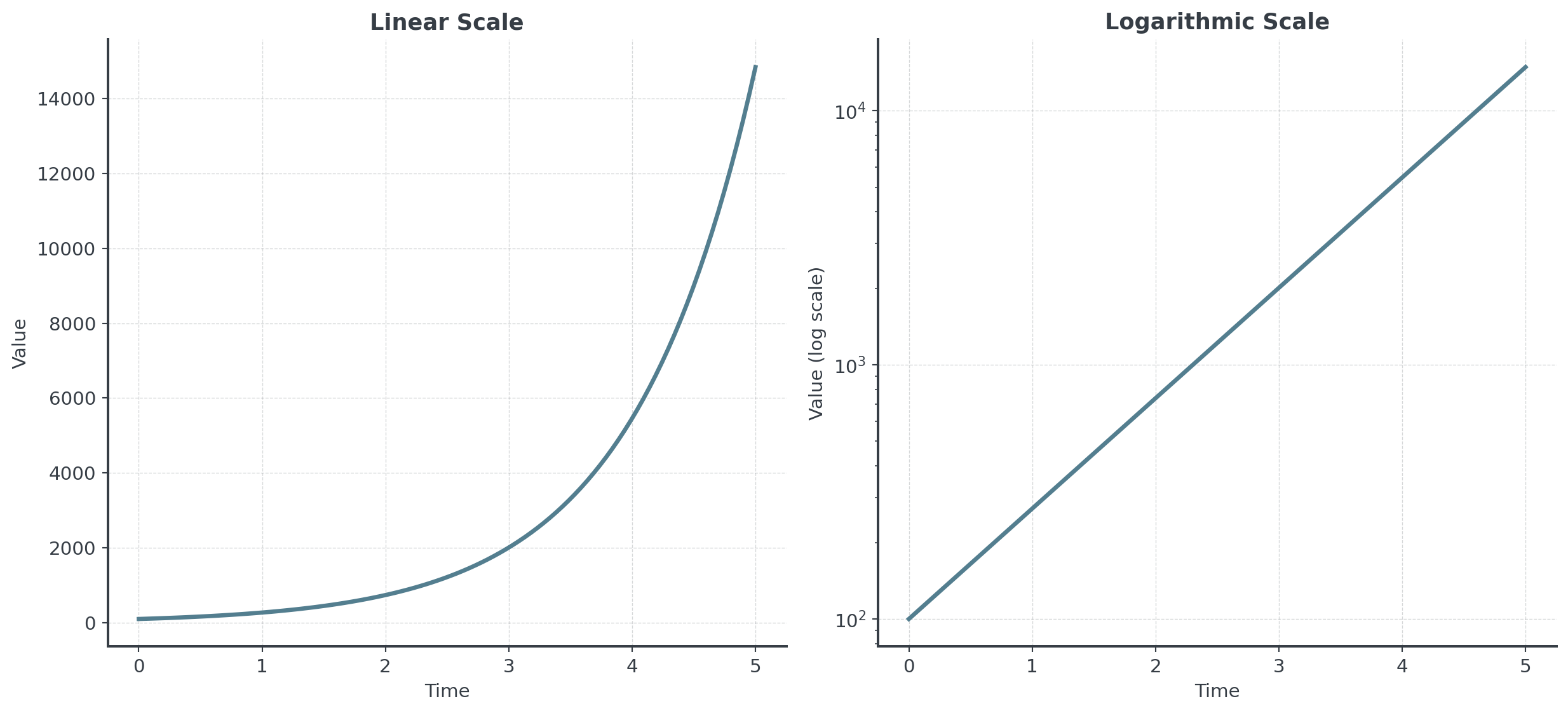
Logarithmic Scales
When exponentials look linear (be careful!)
Mixed Growth Models
Logistic Growth
When exponential growth has limits
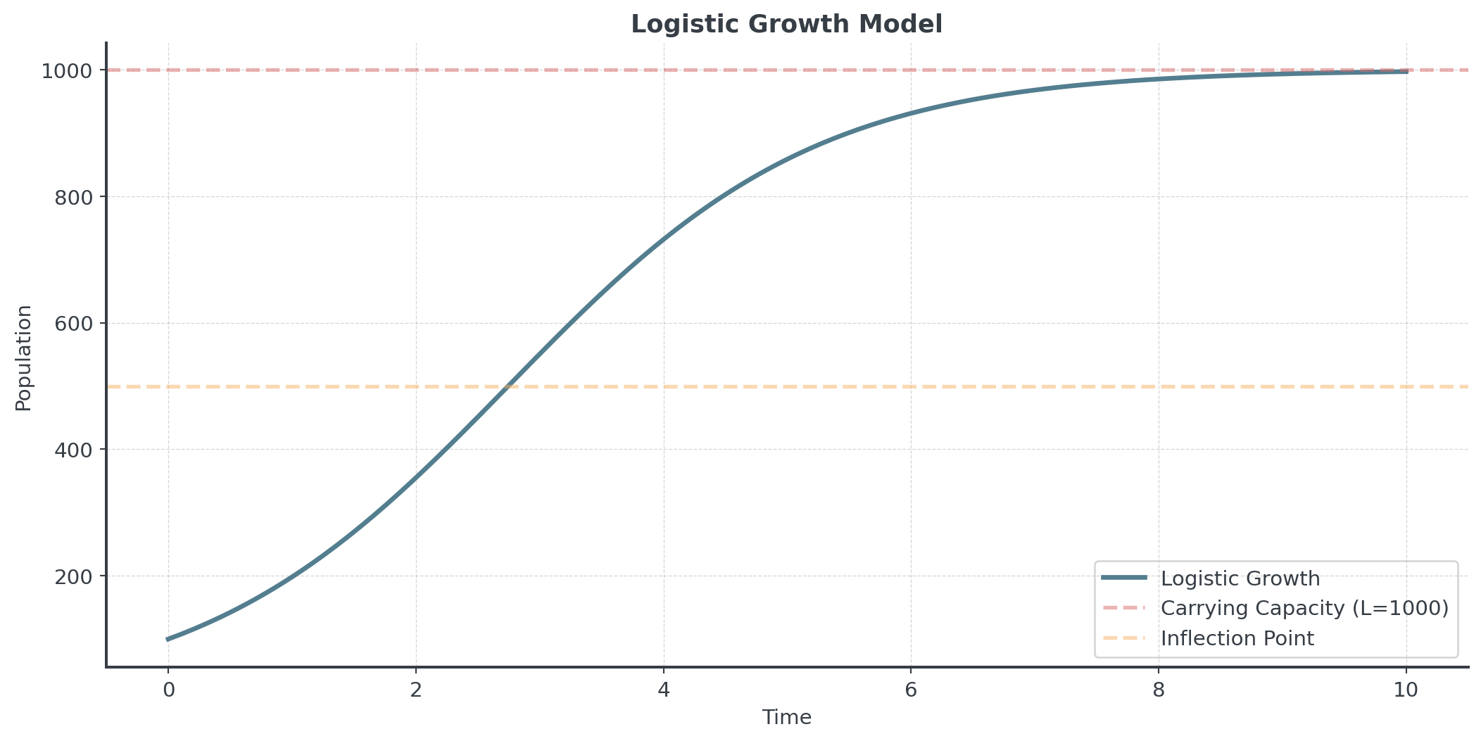
Real populations can’t grow forever. The logistic model:
\[P(t) = \frac{L}{1 + Ae^{-kt}}\]
- \(L\) = carrying capacity (maximum sustainable population)
- \(A\) = related to initial population: \(P(0) = \frac{L}{1+A}\)
- \(k\) = growth rate (how fast it approaches capacity)
- \(t\) = time
Three Phases of Logistic Growth
Phase 1: Slow Start (Lag Phase)
- Population small, resources abundant
- Growth rate increasing but total growth still slow
. . .
Phase 2: Rapid Growth (Exponential-like Phase)
- Population reaches \(\frac{L}{2}\) (inflection point)
- Maximum growth rate occurs here
. . .
Phase 3: Saturation (Plateau Phase)
- Approaching carrying capacity \(L\) as resources become scarce
Logistic Growth Visualization
Real-World Logistic Examples
Where you encounter S-curves in practice
Business & Technology:
- Product adoption: Smartphones, social media platforms
- Market penetration: New products reaching saturation
. . .
Biology & Social:
- Population ecology: Species limited by food/space
- Rumor/news spreading: Reaches everyone who will hear it
. . .
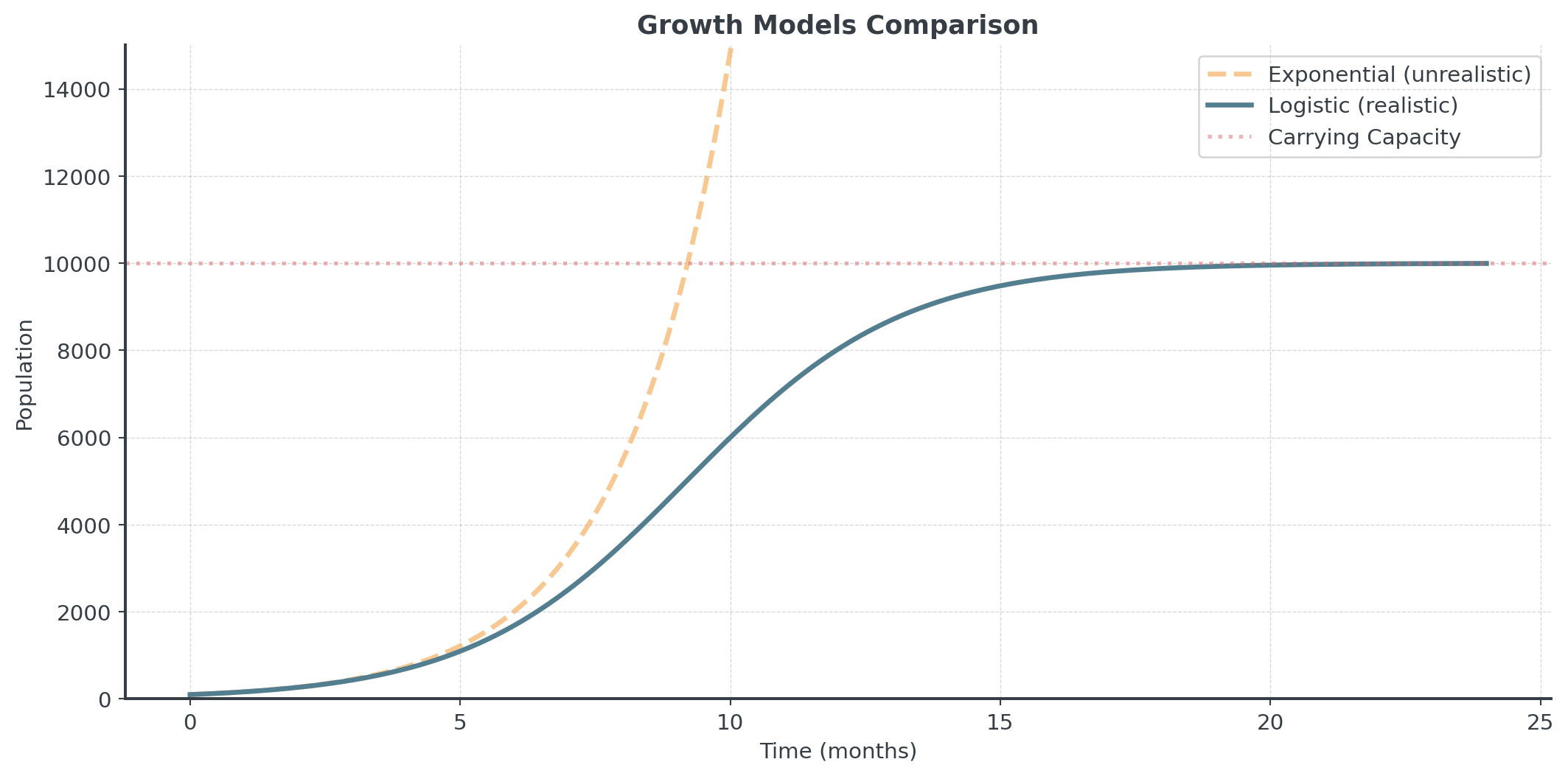
Unlike pure exponential growth (which is unsustainable), logistic growth is realistic. Every real system has limits!
Practice: Logistic Growth Application
Work individually for 5 minutes, then discuss
A new social media platform launches with 100 users. The market can support a maximum of 10,000 users (carrying capacity). The growth follows a logistic model where \(t\) is in months.
\[P(t) = \frac{10000}{1 + 99e^{-0.5t}}\]
- Verify that \(P(0) = 100\) (initial population)
- Calculate the population after 6 months
- After 12 months? What happens as \(t \to \infty\)?
Comparing Growth Models
Exponential vs. Logistic - A visual comparison
Wrap-Up
Key Takeaways
Today’s essential concepts
- Exponentials grow faster than any polynomial eventually
- The base determines the rate of growth or decay
- Natural exponential \(e\) appears in continuous processes
- Compound interest shows the power of exponential growth
- Rule of 70 provides quick intuition for doubling/halving
Final Assessment
5 minutes - Individual work
A new technology startup’s user base is growing exponentially. They started with 1,000 users and now have 4,000 users after 2 years.
Write the exponential growth model \(N(t) = N_0 \cdot b^t\) (find \(b\))
How many users will they have after 5 years?
Is this discrete or continuous growth? What would the continuous model be?
Using the Rule of 70, approximately when will their user base double from the current 4,000?
Final Thought
The Power of Exponentials
Small changes, dramatic effects
A cent doubled daily for 30 days:
- Day 1: €0.01
- Day 10: €5.12
- Day 20: €5,243
- Day 30: €5,368,709
. . .
“The greatest shortcoming of the human race is our inability to understand the exponential function.” - Albert Bartlett