Session 07-06 - Contingency Tables

Section 07: Probability & Statistics

Author

Dr. Nikolai Heinrichs & Dr. Tobias Vlćek

Entry Quiz - 10 Minutes

Quick Review from Session 07-05

Test your understanding of Bayes’ Theorem

State Bayes’ Theorem.
A test has a true positive rate of 80% and a true negative rate of 90%. If the base rate is 10%, calculate the Positive Predictive Value.
What’s the difference between the true positive rate and the Positive Predictive Value?
If the Positive Predictive Value is low but the Negative Predictive Value is high, what does this tell us about the test?

Homework Discussion - 12 Minutes

Your Questions from Session 07-05

Bring Bayes questions and screening interpretation issues.

Formula method vs contingency table method
Interpreting low base rate results

Learning Objectives

What You’ll Master Today

Construct contingency tables from word problems
Complete tables with missing values using row/column relationships
Read probabilities from tables: marginal, joint, conditional
Test independence using table values
Connect tables to Bayes’ theorem and conditional probability
Work with relative frequency tables (percentages instead of counts)

. . .

Contingency tables are a key exam format — expect at least one problem!

Part A: Table Structure

Two-Way Contingency Table

Shows the joint distribution of two categorical variables.

. . .

	\(B\)	\(\bar{B}\)	Total
\(A\)	\(n_{AB}\)	\(n_{A\bar{B}}\)	\(n_A\)
\(\bar{A}\)	\(n_{\bar{A}B}\)	\(n_{\bar{A}\bar{B}}\)	\(n_{\bar{A}}\)
Total	\(n_B\)	\(n_{\bar{B}}\)	\(n\)

. . .

Cells: Joint frequencies (both conditions met)
Row totals: Marginal frequencies for A
Column totals: Marginal frequencies for B
Grand total: \(n\) (bottom-right corner)

Reading Probabilities from Tables

Type	Formula	Where to Look
Marginal	\(P(A)\)	Row total / Grand total
Joint	\(P(A \cap B)\)	Cell / Grand total
Conditional	\(P(A\|B)\)	Cell / Column total

. . .

The most common exam mistake: using the wrong denominator for conditional probabilities!

\(P(A|B)\): denominator is the column total for \(B\)
\(P(B|A)\): denominator is the row total for \(A\)

Example: Market Research

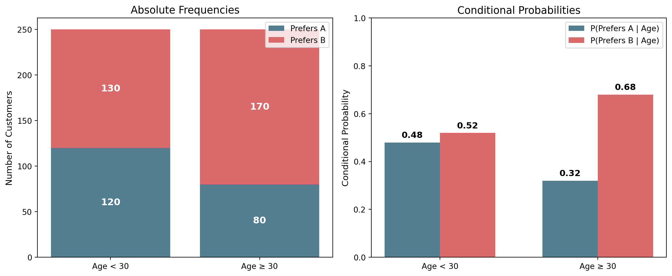
Survey of 500 customers about product preference and age:

	Age < 30	Age ≥ 30	Total
Prefers A	120	80	200
Prefers B	130	170	300
Total	250	250	500

. . .

Calculate:

\(P(\text{Prefers A}) = \frac{200}{500} = 0.40\) (marginal)
\(P(\text{Age} < 30 \cap \text{Prefers A}) = \frac{120}{500} = 0.24\) (joint)
\(P(\text{Prefers A} | \text{Age} < 30) = \frac{120}{250} = 0.48\) (conditional)

Visualizing Contingency Tables

. . .

The right panel shows that preference depends on age — younger customers favour A more.

Part B: Constructing Tables from Word Problems

Strategy for Word Problems

Step-by-Step Approach:

Identify the two variables and their categories
Create empty table with row/column labels and totals
Fill in given values (often percentages → convert to counts)
Use subtraction to complete missing cells
Verify: Row and column totals must match the grand total

Example: Building a Table

In a city of 10,000 residents:

40% are employed
70% are adults (age ≥ 18)
35% are employed adults

. . .

Step 1: Fill in what we know

. . .

	Adult	Minor	Total
Employed	3,500	?	4,000
Not Employed	?	?	6,000
Total	7,000	3,000	10,000

Completing the Table

Step 2: Use subtraction to fill remaining cells

. . .

	Adult	Minor	Total
Employed	3,500	500	4,000
Not Employed	3,500	2,500	6,000
Total	7,000	3,000	10,000

. . .

Now we can answer conditional questions:

\(P(\text{Employed}|\text{Minor}) = \frac{500}{3{,}000} = \frac{1}{6} \approx 0.167\)
\(P(\text{Adult}|\text{Employed}) = \frac{3{,}500}{4{,}000} = 0.875\)

Exam-Style Problem

A company surveyed 200 customers:

60% are satisfied with the product
45% are repeat customers
Of the satisfied customers, 60% are repeat customers

. . .

Step 1: Fill in direct values

. . .

	Repeat	New	Total
Satisfied	?	?	120
Not Satisfied	?	?	80
Total	90	110	200

Solution Continued

Step 2: Use “Of satisfied, 60% are repeat”

\(P(\text{Repeat}|\text{Satisfied}) = 0.60\), so \(72\) repeat AND satisfied

. . .

	Repeat	New	Total
Satisfied	72	48	120
Not Satisfied	18	62	80
Total	90	110	200

. . .

Always read conditional statements carefully: “of the satisfied” means the total number of satisfied is 120, not 200!

Quick Check - 6 Minutes

Building and Reading Tables

Work individually

A company has 300 employees. 180 are in Sales, the rest in Operations. Of the Sales employees, 40% received a bonus. Of Operations employees, 25% received a bonus.

Construct the full contingency table.
Compute \(P(\text{Sales}|\text{Bonus})\).
Are department and bonus independent?

Break - 10 Minutes

Part C: Independence Testing

When Are Variables Independent?

Independence in Tables

Variables A and B are independent if and only if for every cell:

. . .

\[P(A \cap B) = P(A) \cdot P(B)\]

. . .

Equivalently, the expected count under independence is:

. . .

\[E_{ij} = \frac{\text{Row total} \times \text{Column total}}{\text{Grand total}}\]

. . .

If observed \(\neq\) expected in any cell, the variables are NOT independent.

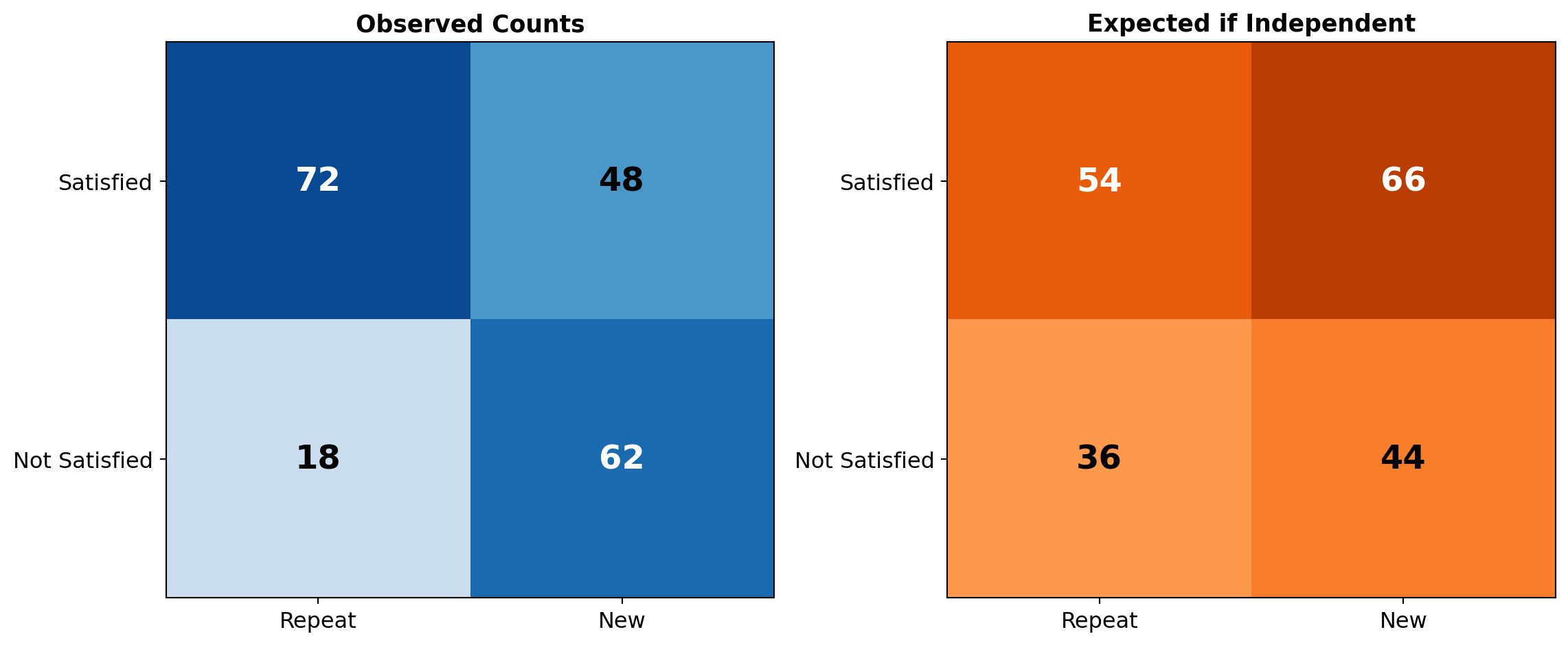
Testing Independence: Example

From our customer survey:

	Repeat	New	Total
Satisfied	72	48	120
Not Satisfied	18	62	80
Total	90	110	200

. . .

Question: If satisfaction and repeat status were independent, what would we expect in the (Satisfied, Repeat) cell?

. . .

\[E = \frac{120 \times 90}{200} = 54\]

Visual: Observed vs Expected

. . .

Large differences between observed and expected → strong evidence against independence.

Interpretation

The data suggests:

Satisfied customers are MORE likely to be repeat customers
\(P(\text{Repeat}|\text{Satisfied}) = \frac{72}{120} = 0.60\)
\(P(\text{Repeat}|\text{Not Satisfied}) = \frac{18}{80} = 0.225\)

. . .

Satisfied customers are about 2.7 times more likely to be repeat customers!

Part D: Connecting to Bayes’ Theorem

Tables and Bayes

Table method from Session 07-05 is exactly this technique!

. . .

Classification as a contingency table:

	Condition (+)	Condition (−)	Total
Predicted +	TP	FP	All +
Predicted −	FN	TN	All −
Total	Condition +	Condition −	Population

Positive Predictive Value = \(P(D|+) = \frac{\text{TP}}{\text{All +}}\) — Bayes via the table!
Negative Predictive Value = \(P(D'|-) = \frac{\text{TN}}{\text{All -}}\)

The Denominator Rule

For conditional prob., the denominator is always the condition total!

\(P(A|B)\) → divide by “all \(B\)” (column total)
\(P(B|A)\) → divide by “all \(A\)” (row total)
\(P(A \cap B)\) → divide by grand total

. . .

Always state the condition in words before choosing the denominator.

Converting Between Approaches

Given: TPR = 90%, TNR = 95%, BR = 2%, Population = 10,000

. . .

	Condition + (200)	Condition − (9,800)	Total
Predicted +	180	490	670
Predicted −	20	9,310	9,330
Total	200	9,800	10,000

. . .

Direct calculations:

Positive Predictive Value = \(\frac{180}{670} \approx 0.269\)
Negative Predictive Value = \(\frac{9{,}310}{9{,}330} \approx 0.998\)

Part E: Relative Frequency Tables

Working with Percentages

Sometimes tables give proportions instead of counts:

	\(B\)	\(B'\)	Total
\(A\)	0.15	0.25	0.40
\(A'\)	0.35	0.25	0.60
Total	0.50	0.50	1.00

. . .

The same rules apply — cells are joint probabilities, margins are marginal probabilities.

\(P(A|B) = \frac{P(A \cap B)}{P(B)} = \frac{0.15}{0.50} = 0.30\)
\(P(B|A) = \frac{P(A \cap B)}{P(A)} = \frac{0.15}{0.40} = 0.375\)

Independence Test with Proportions

From the previous table, test independence:

. . .

\[P(A) \cdot P(B) = 0.40 \times 0.50 = 0.20\]

\[P(A \cap B) = 0.15\]

. . .

\(0.15 \neq 0.20\), so A and B are NOT independent.

. . .

With a relative frequency table, you never need to multiply by a population size — just compare the cell value directly with the product of the marginals.

Converting Between Formats

Question: Given a relative table, how do you get a count table?

. . .

Multiply every entry by the population size!

. . .

If \(n = 200\):

	\(B\)	\(B'\)	Total
\(A\)	\(0.15 \times 200 = 30\)	\(0.25 \times 200 = 50\)	80
\(A'\)	\(0.35 \times 200 = 70\)	\(0.25 \times 200 = 50\)	120
Total	100	100	200

. . .

If a problem gives percentages and asks for counts, pick a convenient total and multiply.

Build and Read Any 2×2 Table

Checklist:

Define event symbols first (e.g., \(A\), \(B\))
Fill totals and directly given values
Subtract to complete missing cells
Verify all four internal cells sum to grand total
Read probabilities with the correct denominator:
- Joint → divide by grand total
- Marginal → row or column total / grand total
- Conditional → divide by the condition’s total

Guided Practice - 20 Minutes

Practice Problem 1

Work in pairs

A survey of 400 employees found:

55% work full-time
40% have a graduate degree
25% work full-time AND have a graduate degree

Construct the contingency table
Find \(P(\text{Grad degree}|\text{Full-time})\)
Find \(P(\text{Full-time}|\text{Grad degree})\)
Are full-time status and graduate degree independent?

Practice Problem 2 (Exam-Style)

Work in pairs

A company produces items at two factories:

Factory A produces 3,000 items, 5% defective
Factory B produces 2,000 items, 8% defective

Construct a contingency table
An item is randomly selected and found defective. What’s the probability it came from Factory A?
What percentage of all items are defective?

Practice Problem 3

In a retail database, let \(K\) = customer bought this month, and \(T\) = customer uses loyalty card.

	\(T\)	\(T'\)	Total
\(K\)	180	120	300
\(K'\)	90	210	300
Total	270	330	600

State in words what each event means: \(T'\), \(K' \cap T\), \(T \setminus K\).
Compute \(P(T \setminus K)\).
Write in words what \(P(T|K')\) means and compute it.

Practice Problem 4

A study reports the following relative frequency table:

	Online	In-Store	Total
Return	0.12	0.03	0.15
Keep	0.48	0.37	0.85
Total	0.60	0.40	1.00

What is the probability that a randomly chosen purchase is an online return?
Given a purchase was returned, what is the probability it was online?
Are purchase channel and return status independent?

Chained Exam Mini-Problem

Work individually, then compare

From a table: total \(n=500\), with \(n_{AB}=90\), row total \(n_A=200\), column total \(n_B=150\).

Compute \(P(A \cap B)\).
Use (a) and totals to compute \(P(A|B)\).
Compare \(P(A \cap B)\) with \(P(A) \cdot P(B)\) and assess independence.

Coffee Break - 10 Minutes

Collaborative Problem-Solving - 20 Minutes

Challenge 1: Campaign Conversion

Think individually (2 min), then work in groups of 3-4

A campaign contacts 800 customers.

320 clicked the email (\(C\))
180 purchased (\(P\))
110 both clicked and purchased

Build the full 2×2 contingency table.
Compute \(P(P|C)\) and \(P(P|C')\).
Test whether clicking and purchasing are independent.
Give one practical marketing interpretation.

Challenge 2: Student Performance

Think individually, then work in groups

A university tracks 600 students across two dimensions: study method (lecture-only vs lecture + tutorial) and exam result (pass vs fail).

360 students attended tutorials in addition to lectures, 480 students passed the exam and of those who attended tutorials, 85% passed

Construct the contingency table.
Compute \(P(\text{Pass}|\text{Lecture only})\).
Are study method and exam result independent?
A student passed. What is the probability they attended tutorials?

Challenge 3: Quality Audit

Think individually, then work in groups

A factory inspector tests items from two production shifts. The following relative frequency table is given:

	Day Shift	Night Shift	Total
Conforming	?	?	?
Non-conforming	0.04	0.06	0.10
Total	0.55	0.45	1.00

Complete the table.
Which shift has the higher non-conforming rate?
If the factory produces 2,000 items per day, construct the count table.

Final Assessment - 5 Minutes

Exit Ticket

Work individually

In a contingency table, where do you find \(P(A \cap B)\)?
If the cell count for \((A, B)\) is 36 and the column total for \(B\) is 120, what is \(P(A|B)\)?
How do you check whether two variables in a table are independent?

Wrap-Up & Key Takeaways

Today’s Essential Concepts

Table structure: Cells = joint, margins = marginal
Reading probabilities: Joint, marginal, conditional — each has a different denominator
Building tables: Fill given values, then subtract to complete
Independence test: Compare observed cell with expected = row% × col% × total
Relative frequency tables: Same rules, no population size needed
Connection to Bayes: Tables provide a visual way to compute Bayes

Next Session Preview

Coming Up: Binomial Distribution

Discrete probability distributions
Binomial formula: \(P(X=k) = \binom{n}{k} p^k (1-p)^{n-k}\)
“Exactly k”, “at most k”, “at least k”
Expected value and variance

. . .

Homework

Complete Tasks 07-06 — practice building and reading contingency tables!