Session 07-04 - Conditional Probability

Section 07: Probability & Statistics

Author

Dr. Nikolai Heinrichs & Dr. Tobias Vlćek

Entry Quiz - 10 Minutes

Quick Review from Session 07-03

Test your understanding of Combinatorics

Calculate \(\binom{8}{3}\)
How many ways can 5 people line up in a row?
A committee of 3 is chosen from 10 people. How many ways?
What’s the probability of getting exactly 3 heads in 5 coin flips? (Use combinations)

Homework Discussion - 12 Minutes

Your Questions from Session 07-03

Let’s resolve any confusion before conditional probability.

Choosing permutations vs combinations
Translating counting results into probabilities
Avoiding overcounting

Learning Objectives

What You’ll Master Today

Define conditional probability: \(P(A|B) = \frac{P(A \cap B)}{P(B)}\)
Apply the multiplication rule: \(P(A \cap B) = P(A|B) \cdot P(B)\)
Construct and use tree diagrams for sequential events
Apply the law of total probability
Test for independence using conditional probability
Compute expectation and variance for discrete random variables

. . .

Conditional probability is heavily tested on the Feststellungsprüfung!

Part A: Conditional Probability Concept

Motivation

Question: A card is drawn from a deck. What’s the probability it’s a king?

. . .

\[P(\text{King}) = \frac{4}{52} = \frac{1}{13}\]

. . .

Question: Given the card is a face card, what’s the probability it’s a king?

. . .

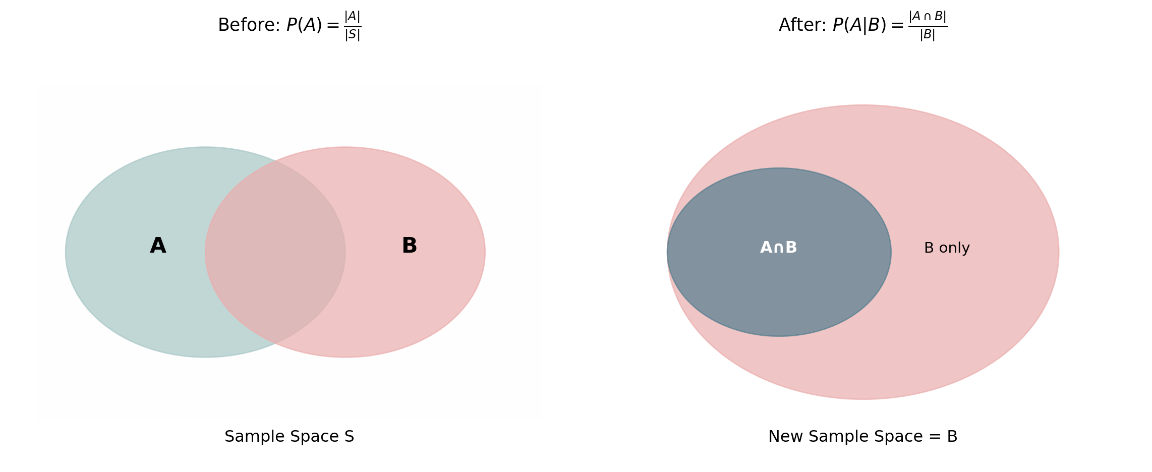
The condition changes the sample space!

\[P(\text{King} | \text{Face card}) = \frac{4}{12} = \frac{1}{3}\]

Conditional Probability Definition

Definition: Conditional Probability

The probability of A given that B has occurred where \(P(B) > 0\).

\[P(A|B) = \frac{P(A \cap B)}{P(B)}\]

. . .

Read “\(P(A|B)\)” as “probability of A given B”

Visual Interpretation

Example Calculation

In a company: 60% work full-time, 30% work full-time AND have a degree.

. . .

Question: What’s the probability an employee has a degree, given they work full-time?

. . .

Let D = has degree, F = full-time

. . .

\[P(D|F) = \frac{P(D \cap F)}{P(F)} = \frac{0.30}{0.60} = 0.50\]

. . .

Given that someone works full-time, there’s a 50% chance they have a degree.

Part B: Multiplication Rule

From Conditional to Joint Probability

Rearranging the definition of the Multiplication Rule:

\[P(A \cap B) = P(A|B) \cdot P(B)\]

. . .

or equivalently:

\[P(A \cap B) = P(B|A) \cdot P(A)\]

. . .

Both formulas give the same result!

Example: Sequential Selection

A box contains 5 red and 3 blue balls. Two balls are drawn without replacement.

Question: What’s the probability both are red?

. . .

Let \(R_1\) = first ball red, \(R_2\) = second ball red

. . .

\[P(R_1 \cap R_2) = P(R_2|R_1) \cdot P(R_1)\]

. . .

\[= \frac{4}{7} \times \frac{5}{8} = \frac{20}{56} = \frac{5}{14}\]

Extended Multiplication Rule

For three or more events:

\[P(A \cap B \cap C) = P(A) \cdot P(B|A) \cdot P(C|A \cap B)\]

. . .

Example: Drawing 3 cards without replacement of a deck of 52 cards. What’s the probability of getting 3 aces?

. . .

\[P(\text{3 aces}) = \frac{4}{52} \times \frac{3}{51} \times \frac{2}{50} = \frac{24}{132,600} = \frac{1}{5,525}\]

. . .

Do you get the idea? We can extend this to any number of events.

Part C: Tree Diagrams

Visual Tool for Sequential Events

Tree diagrams help visualize the multiplication rule.

Branches = outcomes at each stage
Branch labels = probabilities (conditional if sequential)
Multiply along paths = joint probability
Add across paths = union probability

. . .

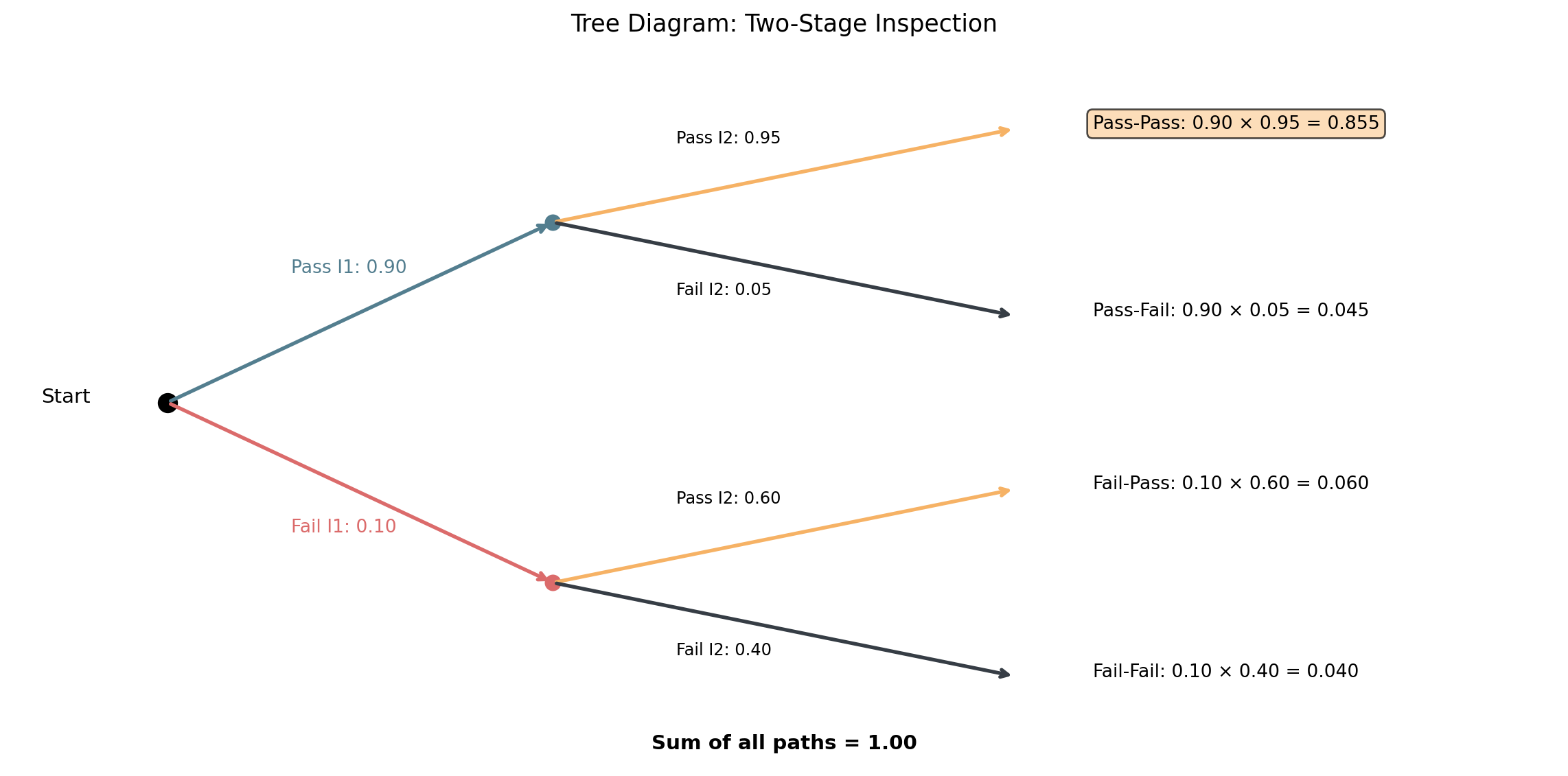
Example: A machine produces items that pass through 2 inspections.

90% pass inspection 1
Of those passing inspection 1: 95% pass inspection 2
Of those failing inspection 1: 60% pass inspection 2

Example: Quality Control

. . .

These diagrams are a great way to visualize the multiplication rule!

Reading Tree Diagrams

From the previous example:

. . .

P(item passes both inspections): Follow Pass-Pass path \[0.90 \times 0.95 = 0.855\]

. . .

P(item passes inspection 2): Add all paths ending with Pass I2 \[0.855 + 0.060 = 0.915\]

. . .

P(passed I1 | passed I2): (We’ll use Bayes for this later!) \[P(I_1|I_2) = \frac{P(I_1 \cap I_2)}{P(I_2)} = \frac{0.855}{0.915} \approx 0.934\]

With vs Without Replacement

Same setup, different dependency structure:

Suppose a bag has 3 red and 2 blue marbles, draw two marbles.

. . .

With replacement:

First red then second red: \(\frac{3}{5}\cdot\frac{3}{5}=\frac{9}{25}\)
Second draw probability stays the same because composition resets.

. . .

Without replacement:

First red then second red: \(\frac{3}{5}\cdot\frac{2}{4}=\frac{3}{10}\)
Second draw probability changes because one marble is removed.

Quick Check - 6 Minutes

Conditional vs Reverse Conditional

Work individually

Given \(P(A)=0.4\), \(P(B)=0.5\), and \(P(A \cap B)=0.2\):

Compute \(P(A|B)\).
Compute \(P(B|A)\).
Explain in one sentence why these two values can differ.

Break - 10 Minutes

Part D: Law of Total Probability

Partitioning the Sample Space

Definition: Law of Total Probability

If events \(B_1, B_2, ..., B_n\) partition the sample space (mutually exclusive and exhaustive):

\[P(A) = \sum_{i=1}^{n} P(A|B_i) \cdot P(B_i)\]

. . .

Common case with two partitions:

\[P(A) = P(A|B) \cdot P(B) + P(A|B') \cdot P(B')\]

Example: Market Segments

A company sells to three market segments:

Segment A: 50% of customers, 20% buy premium
Segment B: 30% of customers, 35% buy premium
Segment C: 20% of customers, 50% buy premium

. . .

Question: What percentage of all customers buy premium?

. . .

\[P(\text{Premium}) = 0.20(0.50) + 0.35(0.30) + 0.50(0.20)\] \[= 0.10 + 0.105 + 0.10 = 0.305\]

. . .

30.5% of customers buy premium products.

Part E: Independence Revisited

Testing Independence

Definition: Independence Test

Events A and B are independent if and only if:

\[P(A|B) = P(A)\]

. . .

Learning B occurred doesn’t change the probability of A!

. . .

Equivalently: \(P(B|A) = P(B)\) or \(P(A \cap B) = P(A) \cdot P(B)\)

Example: Testing Independence

Survey data shows:

\(P(\text{Exercise regularly}) = 0.40\)
\(P(\text{Healthy weight}) = 0.55\)
\(P(\text{Healthy weight}|\text{Exercise}) = 0.70\)

. . .

Question: Are “exercise regularly” and “healthy weight” independent?

. . .

Test: Is \(P(\text{Healthy}|\text{Exercise}) = P(\text{Healthy})\)?
\(0.70 \neq 0.55\)
Conclusion: Events are NOT independent, exercise is associated with healthy weight.

Part F: Expectation and Variance Toolkit

Expected Value

Definition of the Expected Value

For a discrete random variable \(X\) with values \(x_i\) and probabilities \(p_i\):

\[E[X]=\sum_i x_i p_i\]

. . .

Interpretation: long-run average outcome with \(p_i=P(X=x_i)\).

. . .

Although it looks formally difficult, the expected value is something you might feel that has to be true. It simply states that the average outcome is the weighted average of all possible outcomes.

VAR and STD (Recap)

You already know these from Session 07-01:

Descriptive Statistics	Random Variable Notation
\(s^2 = \frac{\sum (x_i - \bar{x})^2}{n-1}\)	\(\mathrm{Var}(X) = E[(X - \mu)^2]\)
\(s = \sqrt{s^2}\)	\(\sigma_X = \sqrt{\mathrm{Var}(X)}\)

. . .

Same idea, new notation: instead of averaging squared deviations from a sample, we take the expected value of squared deviations from \(\mu = E[X]\).

Worked Mini Example

A project has outcomes for weekly profit (in kEUR):

\(x\)	10	20	30
\(P(X=x)\)	0.2	0.5	0.3

. . .

\[E[X]=10(0.2)+20(0.5)+30(0.3)=2+10+9=21\]

. . .

So the expected weekly profit is 21 kEUR.

Linearity and Transformation Rules

Definition: High-Value Rules

For constants \(a,b\):

\[E[aX+b]=aE[X]+b\]

\[\mathrm{Var}(aX+b)=a^2\mathrm{Var}(X)\]

Adding a constant shifts the mean but does not change variance.

. . .

Makes intuitive sense: if you add 100 to every outcome, the mean increases by 100, but the spread of outcomes does not change.

Sum of Independent Variables

If \(X\) and \(Y\) are independent:

\[E[X+Y]=E[X]+E[Y]\]

\[\mathrm{Var}(X+Y)=\mathrm{Var}(X)+\mathrm{Var}(Y)\]

. . .

Example: If \(E[X]=10\), \(\mathrm{Var}(X)=4\) and \(E[Y]=6\), \(\mathrm{Var}(Y)=3\):

\(E[X+Y]=10+6=16\)
\(\mathrm{Var}(X+Y)=4+3=7\) (if independent!)

. . .

Expectation always adds. Variance adds only under independence.

Business Application: Two Campaigns

A and B have random profit contributions \(X\) and \(Y\), independent.

\(E[X]=8\), \(\mathrm{Var}(X)=9\)
\(E[Y]=5\), \(\mathrm{Var}(Y)=4\)

. . .

For total \(T=X+Y\):

\(E[T]=8+5=13\)
\(\mathrm{Var}(T)=9+4=13\)
\(\sigma_T=\sqrt{13}\approx3.61\)

Expectation and Variance Practice

Work individually

Given a random variable with \(E[X]=12\) and \(\mathrm{Var}(X)=5\):

Compute \(E[3X-2]\).
Compute \(\mathrm{Var}(3X-2)\).
If independent \(Y\) has \(E[Y]=4\), \(\mathrm{Var}(Y)=7\), compute \(E[X+Y]\) and \(\mathrm{Var}(X+Y)\).

Guided Practice - 20 Minutes

Practice Problems

Work in pairs

Problem 1: 70% of students study math, 60% study economics, and 45% study both.

Find \(P(\text{Econ}|\text{Math})\)
Find \(P(\text{Math}|\text{Econ})\)
Are these events independent?

Problem 2: Draw a tree diagram for: A bag has 3 red and 2 blue marbles. Two marbles are drawn without replacement. Find \(P(\text{both same color})\).

Chained Exam Mini-Problem

Work individually, then compare

Given \(P(A)=0.50\), \(P(B)=0.30\), and \(P(B|A)=0.60\):

Compute \(P(A\cap B)\).
Use (a) to compute \(P(A|B)\).
Decide whether \(A\) and \(B\) are independent.

Coffee Break - 10 Minutes

Collaborative Problem-Solving - 20 Minutes

Group Challenge: Supplier Reliability

Think individually then work in groups

A company has two suppliers. Let: \(A\) = order from Supplier A and \(O\) = order arrives on time. Given: \(P(A)=0.6\), \(P(O|A)=0.9\), \(P(O|A')=0.75\)

Compute \(P(A \cap O)\) and \(P(A' \cap O)\).
Compute overall on-time probability \(P(O)\).
Compute \(P(A|O)\).
Decide whether on-time arrival is independent of supplier choice.

Final Assessment - 5 Minutes

Exit Ticket

Work individually, then compare

If \(P(A \cap B)=0.18\) and \(P(B)=0.30\), find \(P(A|B)\).
In one sentence, explain the difference between \(P(A|B)\) and \(P(B|A)\).
A bag has 4 red and 1 blue ball. Two draws without replacement. Is \(P(\text{second red}|\text{first red})\) equal to \(P(\text{second red})\)?

Wrap-Up & Key Takeaways

Today’s Essential Concepts

Conditional probability: \(P(A|B) = \frac{P(A \cap B)}{P(B)}\)
Multiplication rule: \(P(A \cap B) = P(A|B) \cdot P(B)\)
Tree diagrams: Multiply along paths, add across paths
Total probability: Sum over all branches
Independence: \(P(A|B) = P(A)\)
Expectation/variance: summarize average outcome and risk

Next Session Preview

Coming Up: Bayes’ Theorem

Reversing conditional probabilities
Prior and posterior probabilities
Medical testing applications (sensitivity, specificity)
Business decision making

. . .

Homework

Complete Tasks 07-04, focus on tree diagrams and conditional probability!