Session 07-07 - Binomial & Geometric Distributions

Section 07: Probability & Statistics

Author

Dr. Nikolai Heinrichs & Dr. Tobias Vlćek

Entry Quiz - 10 Minutes

Quick Review from Session 07-06

Test your understanding of Contingency Tables

From a contingency table, how do you calculate \(P(A|B)\)?
In a table with 200 total, 80 in category A, 60 in category B, and 30 in both. Find \(P(A|B)\).
How do you test if two variables are independent using a table?
A company has 1,000 employees: 600 full-time, 400 with degrees, 280 full-time with degrees. Build the table.

Homework Discussion - 12 Minutes

Your Questions from Session 07-06

Let’s clarify contingency-table logic before distributions.

Marginal vs joint vs conditional probabilities
Denominator selection in conditional probabilities
Independence checks in tables

Learning Objectives

What You’ll Master Today

Identify binomial experiments and their four requirements
Apply the binomial formula: \(P(X=k) = \binom{n}{k} p^k (1-p)^{n-k}\)
Calculate probabilities: “exactly k”, “at most k”, “at least k”
Use the hypergeometric distribution for sampling without replacement
Use the geometric distribution for “first success” problems
Use z-scores to compute normal probabilities

. . .

Binomial distribution problems appear on every Feststellungsprüfung!

Part A: Binomial Experiments

Requirements for Binomial

Fixed number of trials: \(n\) is known in advance
Two outcomes: Success (probability \(p\)) or Failure (probability \(1-p\))
Independence: Trials don’t affect each other
Constant probability: \(p\) is the same for all trials

. . .

Examples:

Flipping a coin 10 times (heads = success)
Testing 50 products (defective = success)
Surveying 100 customers (satisfied = success)

The Binomial Formula

Binomial Distribution

\[P(X = k) = \binom{n}{k} p^k (1-p)^{n-k}\]

. . .

Where:

\(n\) = number of trials
\(k\) = number of successes
\(p\) = probability of success on each trial
\(\binom{n}{k} = \frac{n!}{k!(n-k)!}\) = number of arrangements

Understanding the Formula

It is not too difficult to understand:

\[P(X = k) = \underbrace{\binom{n}{k}}_{\text{arrangements}} \times \underbrace{p^k}_{\text{k successes}} \times \underbrace{(1-p)^{n-k}}_{\text{n-k failures}}\]

. . .

Example: In 5 coin flips, \(P(\text{exactly 3 heads})\)?

. . .

\[P(X=3) = \binom{5}{3} \times (0.5)^3 \times (0.5)^2 = 10 \times 0.125 \times 0.25 = 0.3125\]

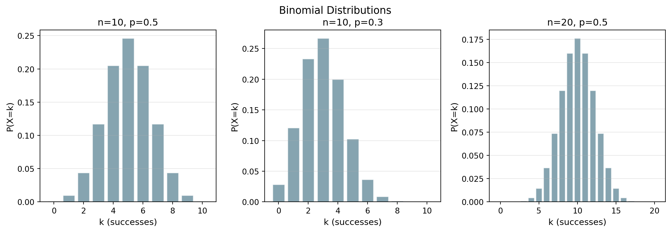
Binomial Distribution Visualization

. . .

When \(p = 0.5\) the distribution is symmetric. When \(p < 0.5\) it is right-skewed. Larger \(n\) makes the distribution more spread out.

Expected Value and Variance

Binomial Mean and Variance

Expected value (mean): \(\mu = E[X] = np\)
Variance: \(\sigma^2 = np(1-p)\)
Standard deviation: \(\sigma = \sqrt{np(1-p)}\)

. . .

Example: If \(n=100\) and \(p=0.3\):

Expected successes: \(\mu = 100 \times 0.3 = 30\)
Standard deviation: \(\sigma = \sqrt{100 \times 0.3 \times 0.7} = \sqrt{21} \approx 4.58\)

Part B: Common Probability Questions

Three Types of Questions

These are the types you will likely see on the exam

Question Type	Formula
Exactly k	\(P(X = k)\)
At most k	\(P(X \leq k) = \sum_{i=0}^{k} P(X=i)\)
At least k	\(P(X \geq k) = 1 - P(X \leq k-1)\)

. . .

For “at least” problems, use the complement rule as it saves you from summing many terms!

Wording Decoder (Exam Language)

Let’s extend the table from the previous slide:

. . .

Phrase	Mathematical form
exactly \(k\)	\(P(X=k)\)
at most \(k\)	\(P(X \le k)\)
at least \(k\)	\(P(X \ge k) = 1 - P(X \le k-1)\)
between \(a\) and \(b\) (inclusive)	\(P(a \le X \le b)\)
first success on trial \(n\)	geometric: \((1-p)^{n-1}p\)

. . .

Always check whether endpoints are included in words like “between”, “at most”, and “at least”.

Example: Quality Control

A machine produces items with 8% defect rate. In a batch of 15 items:

\(P(\text{exactly 2 defective})\)

. . .

\(P(X=2) = \binom{15}{2} (0.08)^2 (0.92)^{13} = 105 \times 0.0064 \times 0.326 \approx 0.219\)

. . .

\(P(\text{at most 1 defective})\)

. . .

\[P(X \leq 1) = P(X=0) + P(X=1)\] \[\binom{15}{0}(0.08)^0(0.92)^{15} + \binom{15}{1}(0.08)^1(0.92)^{14} = 0.659\]

Example Continued

\(P(\text{at least 2 defective})\)

. . .

\[P(X \geq 2) = 1 - P(X \leq 1) = 1 - 0.659 = 0.341\]

. . .

\(P(\text{between 1 and 3 defective, inclusive})\)

. . .

\[P(1 \leq X \leq 3) = P(X=1) + P(X=2) + P(X=3)\] \[\approx 0.373 + 0.219 + 0.085 = 0.677\]

. . .

Do you get the idea? We can compute any probability of interest using the binomial formula.

Quick Check - 6 Minutes

Binomial Setup and Calculation

Work individually

A fair die is rolled 10 times. Let “success” = rolling a 6. Name \(n\) and \(p\).
Compute \(P(X = 0)\) for the setting in question 1.
Translate “at least two sixes in 10 rolls” into a complement expression.

Break - 10 Minutes

Part C: Hypergeometric Distribution

When to Use Hypergeometric

The binomial assumes independent trials (with replacement). But what if we draw without replacement from a finite population?

. . .

Hypergeometric Setup

Use the hypergeometric distribution when:

Population size is fixed: \(N\)
There are \(K\) “success” items in the population
We draw \(n\) items without replacement
We ask for exactly \(k\) successes in the sample

Hypergeometric Formula

Definition: Hypergeometric Probability

\[P(X=k)=\frac{\binom{K}{k}\binom{N-K}{n-k}}{\binom{N}{n}}\]

. . .

Where:

\(N\) = population size
\(K\) = number of successes in population
\(n\) = sample size (drawn without replacement)
\(k\) = successes in sample

Binomial vs Hypergeometric

Feature	Binomial	Hypergeometric
Typical wording	“in 20 trials”	“from a lot of 200 items”
Replacement	With/ Large population)	Without
Independence	Yes	No
Formula	\(\binom{n}{k}p^k(1-p)^{n-k}\)	\(\frac{\binom{K}{k}\binom{N-K}{n-k}}{\binom{N}{n}}\)

. . .

If sampling is without replacement from a finite population, check whether hypergeometric is the correct model before using binomial.

Worked Example: Quality Control

A lot has \(N=50\) items, with \(K=8\) defective. Sample \(n=5\) items without replacement.

. . .

Question: What is \(P(X=2)\)?

. . .

\[P(X=2)=\frac{\binom{8}{2}\binom{42}{3}}{\binom{50}{5}} = \frac{28 \times 11{,}480}{2{,}118{,}760} \approx 0.152\]

Worked Example: Team Selection

From 18 applicants, 7 are international. Choose 5 without replacement.

. . .

Question: What is the probability of exactly 2 international students?

. . .

\[P(X=2)=\frac{\binom{7}{2}\binom{11}{3}}{\binom{18}{5}} = \frac{21 \times 165}{8{,}568} = \frac{3{,}465}{8{,}568} \approx 0.404\]

. . .

If the population is very large compared with the sample, hypergeometric probabilities are close to binomial with \(p = K/N\).

Visualizing Both Distributions

. . .

For small samples from large populations, the two distributions are nearly identical.

Part D: Geometric Distribution

Waiting for First Success

The probability that the first success occurs on trial \(n\):

\[P(X = n) = (1-p)^{n-1} \cdot p\]

Where \(p\) = probability of success on each trial.

. . .

Example: A salesperson has a 20% chance of making a sale on each call. What’s the probability the first sale is on the 4th call?

. . .

\[P(X=4) = (0.8)^3 \times 0.2 = 0.512 \times 0.2 = 0.1024\]

Geometric: Key Formulas

For \(X \sim \text{Geometric}(p)\):

Formula	Use Case
\(P(X=n) = (1-p)^{n-1}p\)	First success on trial \(n\)
\(P(X \le n) = 1 - (1-p)^n\)	At least one success within \(n\) trials
\(P(X > n) = (1-p)^n\)	No success in first \(n\) trials
\(E[X] = \frac{1}{p}\)	Expected number of trials

. . .

Example: If \(p = 0.25\), on average how many trials until first success?

. . .

\[E[X] = \frac{1}{0.25} = 4 \text{ trials}\]

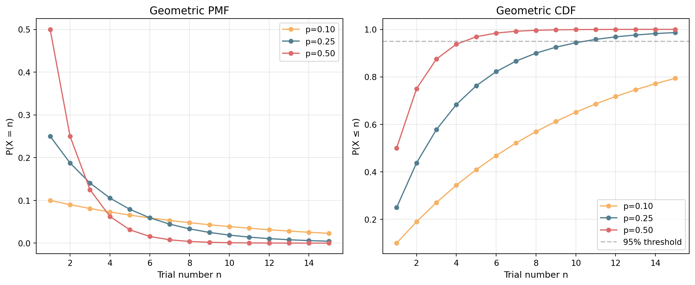
Geometric Visualization

. . .

Higher \(p\) → first success comes sooner. The CDF shows how quickly you reach a target probability.

Exam-Style Example

A machine produces defective items with probability 0.05.

\(P(\text{first defective item is the 10th produced})\)

. . .

\[P(X=10) = (0.95)^9 \times 0.05 = 0.631 \times 0.05 = 0.0316\]

. . .

\(P(\text{first defective item within first 5 items})\)

. . .

\[P(X \leq 5) = 1 - (0.95)^5 = 1 - 0.774 = 0.226\]

Solving for Minimum n (Exam) I

Question: How many items must be checked so that the probability of finding at least one defective item is at least 95%?

. . .

Given \(p=0.05\):

. . .

\[1-(1-p)^n \geq 0.95 \quad \Rightarrow \quad (0.95)^n \leq 0.05\]

. . .

Take logarithms:

\[n \cdot \ln(0.95) \leq \ln(0.05)\]

. . .

Solving for Minimum n (Exam) II

Because \(\ln(0.95) < 0\), the inequality flips when dividing:

. . .

\[n \geq \frac{\ln(0.05)}{\ln(0.95)} \approx 58.4\]

. . .

\[\boxed{n = 59}\]

. . .

Always round up for minimum required sample size — trials are discrete!

Memoryless Property

This is important, also for your life:

For geometric \(X\):

\[P(X > m + n \mid X > m) = P(X > n)\]

If no success has happened yet, the process “restarts” probabilistically.

. . .

Example: A support agent closes tickets with probability \(p=0.25\) per call. Given no closure in the first 4 calls, what is the probability of no closure in the next 3 calls?

. . .

\[P(X>7 \mid X>4) = P(X>3) = (0.75)^3 \approx 0.422\]

Part E: Normal Distribution with z-Scores

Standardization

If \(X \sim N(\mu, \sigma)\), then:

\[Z = \frac{X - \mu}{\sigma} \sim N(0,1)\]

. . .

Use this to convert any normal probability into a standard normal probability!

. . .

One table, the standard normal table, is enough for all normal distributions!

Typical Probability Conversions

Question	Convert to Z-form
\(P(X \le a)\)	\(P\!\left(Z \le \frac{a-\mu}{\sigma}\right)\)
\(P(X \ge a)\)	\(1 - P\!\left(Z \le \frac{a-\mu}{\sigma}\right)\)
\(P(a \le X \le b)\)	\(P\!\left(\frac{a-\mu}{\sigma} \le Z \le \frac{b-\mu}{\sigma}\right)\)

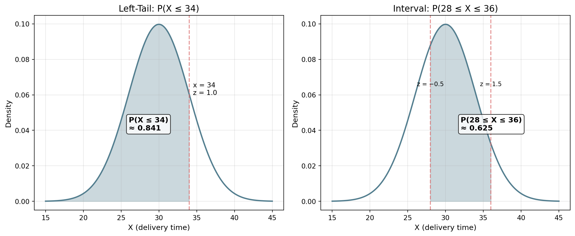
Worked Example: Left-Tail Probability

Normal delivery times with mean 30 min and standard deviation 4 min.

Question: Find \(P(X \le 34)\).

. . .

\[z = \frac{34 - 30}{4} = 1\]

. . .

\[P(X \le 34) = P(Z \le 1) \approx 0.8413\]

Worked Example: Interval Probability

Using the same distribution, find \(P(28 \le X \le 36)\).

. . .

\[z_1 = \frac{28 - 30}{4} = -0.5, \quad z_2 = \frac{36 - 30}{4} = 1.5\]

. . .

\[P(28 \le X \le 36) = P(-0.5 \le Z \le 1.5)\]

. . .

\[\approx 0.9332 - 0.3085 = 0.6247\]

Reverse Question (Quantile)

Exam scores are normal with \(\mu = 70\), \(\sigma = 10\).

Question: What score marks the top 10%?

. . .

Need \(P(X \le x) = 0.90\), so \(z_{0.90} \approx 1.2816\).

. . .

\[x = \mu + z \cdot \sigma = 70 + 1.2816 \times 10 \approx 82.8\]

. . .

So the cutoff is about 83 points.

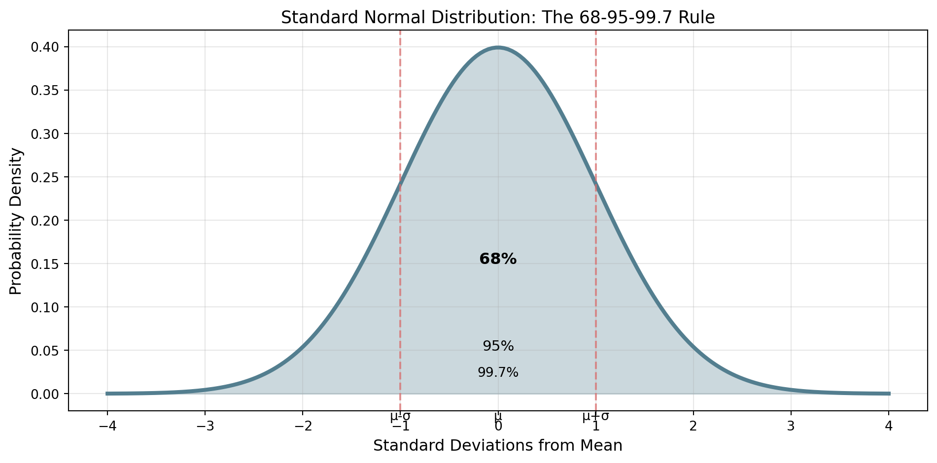
Normal Distribution Visualization

. . .

No worries. You don’t need to know the Z-table by heart. If it is part of the exam it will be given. But we figure it is not going to be an exam task!

Guided Practice - 20 Minutes

Practice Problem 1

Work in pairs

A multiple choice test has 20 questions with 4 options each. A student guesses randomly on all questions.

What’s the probability of getting exactly 5 correct?
What’s the probability of getting at least 8 correct?
What’s the expected number of correct answers?
What’s the standard deviation?

Practice Problem 2

Work in pairs

A company’s call center receives calls with 15% conversion rate.

In 10 calls, what’s the probability of exactly 2 conversions?
In 10 calls, what’s the probability of at least 1 conversion?
What’s the probability that the first conversion is on the 5th call?
On average, how many calls until the first conversion?

Practice Problem 3 (Hypergeometric)

Work in pairs

A box contains 30 light bulbs, of which 6 are defective. A sample of 4 is drawn without replacement.

What is the probability of exactly 1 defective bulb?
What is the probability of no defective bulbs?
What is the probability of at least 1 defective bulb?

Practice Problem 4 (Normal)

Work in pairs

The weight of cereal boxes is normally distributed with \(\mu = 500\)g and \(\sigma = 12\)g.

What proportion of boxes weigh less than 480g?
What proportion weigh between 490g and 520g?
What weight is exceeded by only 5% of boxes?

Chained Exam Mini-Problem

Work individually, then compare

A process has success probability \(p = 0.10\) per trial.

Compute \(P(\text{at least one success in 8 trials})\).
Find the minimum \(n\) such that \(P(\text{at least one success}) \ge 0.95\).
Explain why part (b) must be rounded up.

Coffee Break - 10 Minutes

Collaborative Problem-Solving - 20 Minutes

Challenge 1: Sales Conversion

Think individually (2 min), then work in groups of 3-4

A sales rep has conversion probability \(p = 0.18\) per call.

In 12 calls, compute the probability of exactly 3 conversions.
In 12 calls, compute the probability of at least 1 conversion.
Find the minimum number of calls needed for at least one conversion with probability \(\ge 97\%\).
Explain in one sentence why question 3 requires rounding up.

Challenge 2: Warranty Claims

Think individually, then work in groups

A manufacturer knows that 4% of products have a defect. A retailer receives a shipment of 40 products and selects 6 at random for inspection (without replacement). Assume exactly 2 of the 40 products are defective.

Is this a binomial or hypergeometric problem? Justify.
Compute \(P(\text{exactly 1 defective in the sample})\).
Compute \(P(\text{no defectives in the sample})\).
If the retailer finds no defectives, should they conclude the shipment is defect-free? Discuss.

Challenge 3: Mixed Distribution

Think individually, then work in groups

A taxi company’s ride durations are normally distributed with \(\mu = 15\) min and \(\sigma = 5\) min. On each ride, the driver has a 30% chance of receiving a tip (independent of ride length).

What fraction of rides last more than 20 minutes?
In 8 rides, what is the probability of receiving exactly 3 tips?
On average, how many rides until the first tip?
Find the minimum number of rides so that \(P(\text{at least one tip}) \ge 0.99\).

Final Assessment - 5 Minutes

Exit Ticket

Work individually

For \(X \sim \text{Binomial}(n=12, p=0.3)\), write the formula for \(P(X=4)\).
Write one expression for \(P(X \ge 1)\) in terms of \(n\) and \(p\).
If a minimum required sample size gives \(n \ge 14.2\), what integer must you choose?

Wrap-Up & Key Takeaways

Today’s Essential Concepts

Binomial formula: \(P(X=k) = \binom{n}{k}p^k(1-p)^{n-k}\)
Binomial parameters: \(\mu = np\), \(\sigma = \sqrt{np(1-p)}\)
Three question types: Exactly k, at most k, at least k (complement!)
Hypergeometric: Without replacement from finite populations
Geometric: \((1-p)^{n-1} \cdot p\) for first success on trial \(n\)
Minimum n problems: Use logarithms, always round up
z-scores: Convert any normal to standard normal for table lookup

Next Session Preview

Coming Up: Mock Exam 2

Full 180-minute exam simulation
All Section 07 topics covered
Practice under exam conditions

. . .

Homework

Complete Tasks 07-07 and focus on binomial calculation practice and minimum-\(n\) problems!