Session 04-01 - Polynomial Functions
Section 04: Advanced Functions
Entry Quiz - 10 Minutes
Review from Section 03
Work individually for 5 minutes, then discuss with the class (5 minutes)
Find the vertex of \(f(x) = 2x^2 - 8x + 3\)
If \(f(x) = 2x + 1\) and \(g(x) = x^2\), find \((f \circ g)(3)\)
Given the transformation \(h(x) = -2f(x - 3) + 4\), describe all transformations applied to \(f(x)\)
Find the inverse of \(f(x) = 3x - 5\)
Homework Discussion - 15 Minutes
Your questions from the Mock Exams
Focus on mock exam preparation and key concepts
- Which problems from the mock exam were most challenging?
- Common mistakes with composition and inverse functions
- Graph interpretation challenges
- Business application questions
. . .
Polynomials will extend these concepts to more complex business scenarios!
Learning Objectives
Today
By the end of this session, you will be able to:
- Identify polynomial functions and their key characteristics
- Analyze end behavior using degree and leading coefficient
- Find zeros and determine their multiplicities
- Sketch polynomial graphs from factored form
- Model business scenarios with polynomial functions
- Apply the Intermediate Value Theorem to locate zeros
Polynomial Basics
What is a Polynomial?
Building on our function knowledge
A polynomial function has the form:
\[P(x) = a_nx^n + a_{n-1}x^{n-1} + ... + a_1x + a_0\]
- \(a_n \neq 0\) (leading coefficient)
- \(n\) is a non-negative integer (degree)
- All exponents are whole numbers
. . .
- Linear: polynomials of degree 1, Quadratic: polynomials of degree 2
- Now we explore degree 3 and higher!
Polynomial Vocabulary
Key terminology you need to know
Structural Terms:
Degree: highest power of \(x\)
Leading: highest power coefficient
Constant term: \(a_0\)
Standard: descending powers
Examples:
- \(P(x) = 3x^4 - 2x^2 + x - 7\)
- Degree: 4
- Leading coefficient: 3
- Constant term: -7
. . .
TipQuick Check
Is \(f(x) = \frac{1}{x} + x^2\) a polynomial? No! The term \(\frac{1}{x} = x^{-1}\) has a negative exponent.
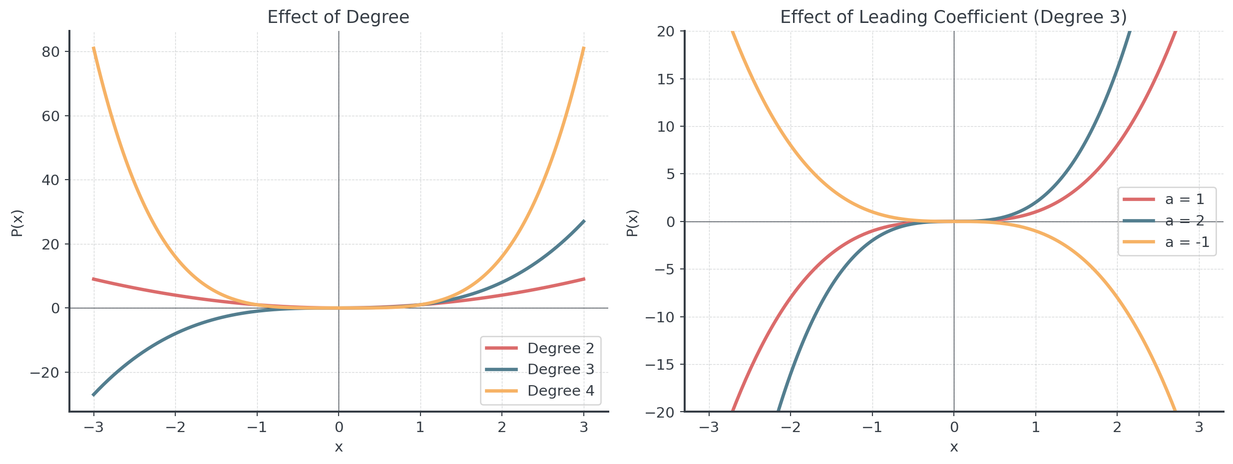
Degree and Leading Coefficient
These two values determine the big picture
The degree tells us:
- Maximum number of zeros
- Maximum number of turning points (degree - 1)
- Overall shape complexity
The leading coefficient determines:
- End behavior direction
- Vertical stretch/compression
Degree and Leading Coefficient II
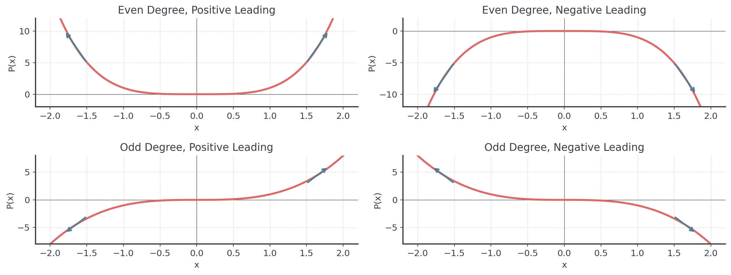
End Behavior Analysis
Understanding End Behavior
What happens as \(x \to \pm\infty\)?
. . .
End behavior depends on:
- Degree (even or odd)
- Sign of leading coefficient (positive or negative)
. . .
Even Degree:
- Both ends go in same direction
- Positive \(a_n\): both up ↗↗
- Negative \(a_n\): both down ↘↘
Odd Degree:
- Ends go in opposite directions
- Positive \(a_n\): down-up ↘↗
- Negative \(a_n\): up-down ↗↘
End Behavior Patterns
The four fundamental patterns
Break - 10 Minutes
Zeros and Their Multiplicities
Finding Zeros
Where the polynomial crosses or touches the x-axis
A zero of \(P(x)\) is a value \(c\) where \(P(c) = 0\). To find zeros:
- Factoring (when possible)
- Quadratic formula (for degree 2 factors)
- Rational Root Theorem (for rational zeros)
- Graphing (approximate locations)
- Calculator (for precise values)
. . .
TipFundamental Theorem of Algebra
A polynomial of degree \(n\) has exactly \(n\) zeros (counting multiplicities and complex zeros).
Intermediate Value Theorem
The Theorem
A tool for finding zeros: Intermediate Value Theorem (IVT)
If \(P(x)\) is continuous on \([a, b]\) and \(P(a) \cdot P(b) < 0\), then there exists at least one \(c\) in \((a, b)\) where \(P(c) = 0\)
. . .
In simple terms:
- If the function is negative at one point
- And positive at another point
- It must cross zero somewhere in between!
. . .
IVT guarantees at least one zero exists but doesn’t tell us exactly where or how many!
Applying IVT
Locating zeros systematically
Example: Show that \(P(x) = x^3 - 2x - 5\) has a zero in \([2, 3]\)
. . .
Solution:
- \(P(2) = 8 - 4 - 5 = -1\) (negative)
- \(P(3) = 27 - 6 - 5 = 16\) (positive)
- Since \(P(2) < 0\) and \(P(3) > 0\), IVT guarantees a zero exists!
. . .
Business Application: Use IVT to prove break-even points exist when you know profit is negative at low production and positive at high production.
More complicated: Rational Zeros
Which “easy” numbers make our polynomial equal zero?
Consider any polynomial with integer coefficients, like:
\[P(x) = 2x^3 - 5x^2 + x + 2\]
. . .
Question: What values of \(x\) make \(P(x) = 0\)?
. . .
Some zeros might be “messy” (like \(\sqrt{2}\) or complex numbers), but some might be “easy” rational numbers (fractions).
. . .
NoteWhy This Matters?
- Rational zeros are exact and easy to work with
- They help us factor polynomials completely
The Rational Root Theorem
Instead of guessing randomly, use a systematic approach
The Rule: If our polynomial has integer coefficients, then any rational zero \(\frac{p}{q}\) (in lowest terms) must follow a pattern.
- \(p\) (numerator) must divide the constant term
- \(q\) (denominator) must divide the leading coefficient
. . .
ImportantWhy p and q?
- \(p\) (numerator) comes from the constant term - the “ending” of the polynomial
- \(q\) (denominator) comes from the leading coefficient - the “beginning” of the polynomial
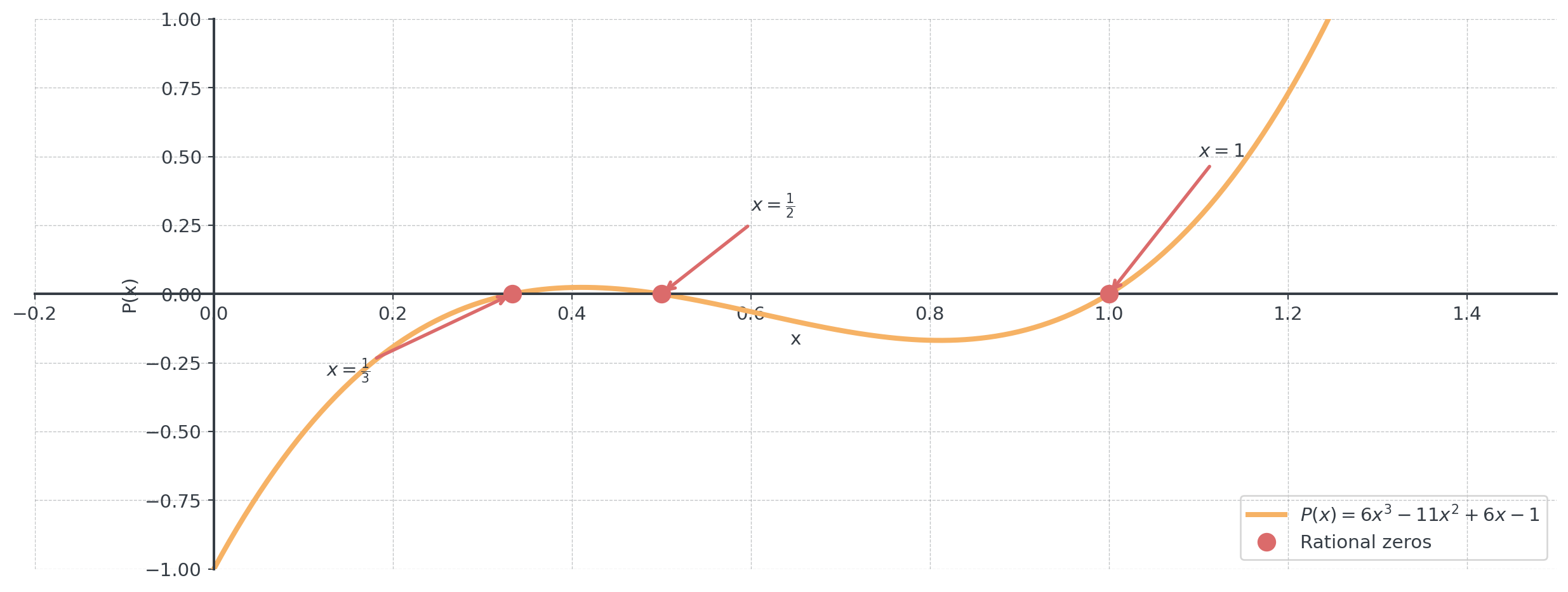
Step 1: Find the p and q Options
Let’s use our example: \(P(x) = 6x^3 - 11x^2 + 6x - 1\)
Constant term (the number without \(x\)): -1
- Factors of -1: \(\pm 1\)
- Possible values for \(p\): \(\pm 1\)
Leading coefficient (number in front of highest power): 6
- Factors of 6: \(\pm 1, \pm 2, \pm 3, \pm 6\)
- Possible values for \(q\): \(\pm 1, \pm 2, \pm 3, \pm 6\)
. . .
See the Difference?
Step 2: Create All Combinations
Mix and match the p and q values
All possible \(\frac{p}{q}\) combinations:
From \(p \in \{\pm 1\}\) and \(q \in \{\pm 1, \pm 2, \pm 3, \pm 6\}\):
\[\frac{\pm 1}{\pm 1}, \frac{\pm 1}{\pm 2}, \frac{\pm 1}{\pm 3}, \frac{\pm 1}{\pm 6}\]
. . .
TipSmart Testing Order
Start with simple fractions: \(\pm 1\), then try: \(\pm \frac{1}{2}, \pm \frac{1}{3}, \pm \frac{1}{6}\)
Step 3: Test the Candidates
Substitute each \(\frac{p}{q}\) candidate into the polynomial
\[P(1) = 6(1)^3 - 11(1)^2 + 6(1) - 1 = 0 \checkmark\]
\[P(\frac{1}{2}) = 6(\frac{1}{2})^3 - 11(\frac{1}{2})^2 + 6(\frac{1}{2}) - 1 = 0 \checkmark\]
\[P(\frac{1}{3}) = 6(\frac{1}{3})^3 - 11(\frac{1}{3})^2 + 6(\frac{1}{3}) - 1 = 0 \checkmark\]
. . .
Result: The rational zeros are \(x = 1\), \(x = \frac{1}{2}\), and \(x = \frac{1}{3}\)
. . .
The theorem doesn’t guarantee these will be zeros - it just tells us which ones are worth testing!
Visualizing Our Example
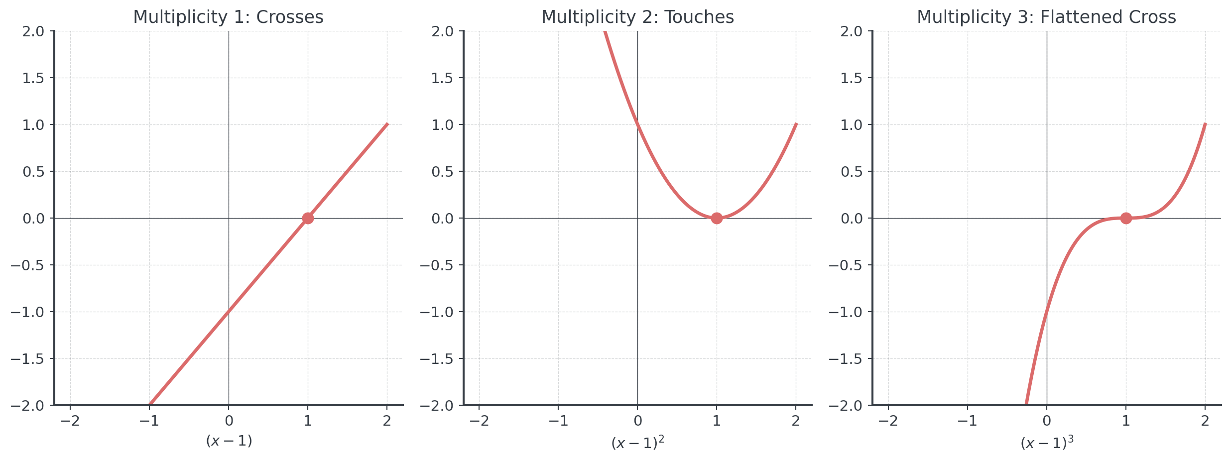
Understanding Multiplicity
How many times a zero appears
If \((x - c)^m\) is a factor of \(P(x)\), then \(c\) has multiplicity \(m\)
Behavior at zeros:
- Odd multiplicity: Graph crosses x-axis
- Even multiplicity: Graph touches x-axis (bounces off)
- Higher multiplicity: Flatter near the zero
. . .
- Linear \(y = x - 1\): The 0 at \(x = 1\) has multiplicity 1 (odd) → crosses the x-axis
- Quadratic \(y = (x - 1)^2\): 0 at \(x = 1\) has multiplicity 2 (even) → touches x-axis and bounces off
- This is the same concept! Polynomials just extend this pattern to higher multiplicities.
Understanding Multiplicity II
Factored Form Insights
Reading the story from the factors
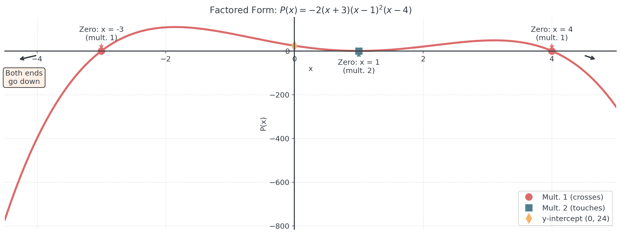
Given: \(P(x) = -2(x + 3)(x - 1)^2(x - 4)\)
What can we determine?
- Zeros: \(x = -3\) (mult. 1), \(x = 1\) (mult. 2), \(x = 4\) (mult. 1)
- Degree: \(1 + 2 + 1 = 4\) (even)
- Leading coefficient: \(-2\) (negative)
- End behavior: Both down ↘↘
- y-intercept: \(P(0) = -2(3)(-1)^2(-4) = 24\)
Factored Form Insights II
Sketching from Factored Form
A systematic approach
Step-by-step process:
- Identify zeros and multiplicities
- Determine end behavior
- Find y-intercept
- Plot key points
- Connect smoothly, respecting multiplicities
. . .
Between zeros, the polynomial doesn’t cross the x-axis. Use test points to determine if the graph is above or below the x-axis in each interval.
Guided Practice - 25 Minutes
Individual Exercise Block I
Work alone for 5 minutes, then discuss for 5 minutes
- Analyze the polynomial \(P(x) = -x^4 + 5x^2 - 4\):
- Identify the degree and leading coefficient
- Describe the end behavior
- Factor completely and find all zeros with their multiplicities
- Sketch the graph showing all key features
Individual Exercise Block II
Work alone for 5 minutes, then discuss for 5 minutes
- Given \(Q(x) = (x + 2)^2(x - 1)(x - 3)^3\):
- List all zeros and their multiplicities
- Determine the degree
- If the leading coefficient becomes negative, how does the graph change?
Coffee Break - 15 Minutes
Business Applications
Real-World Polynomial Applications
Where do we see polynomials in business?
- Revenue functions: Price depends on quantity (non-linear demand)
- Cost functions: With economies and diseconomies of scale
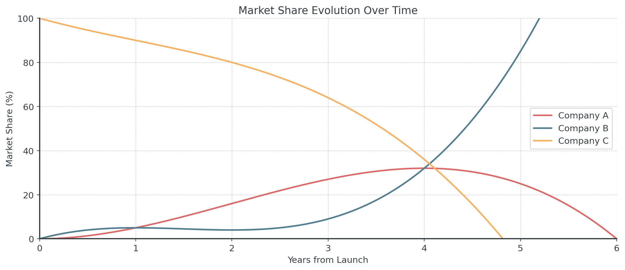
- Market share models: Competition dynamics over time
- Multi-product interactions: How products affect each other
- Break-even analysis: Multiple equilibrium points
. . .
Let’s do this with an example!
TechCo Case Study - Part I
When products interact
TechCo produces three related products with profit function:
\[P(x) = -x^3 + 12x^2 - 35x + 24\]
where \(x\) is production level (thousands of units).
. . .
Business Question: At what levels does the company break even?
. . .
Mathematical Task: Solve \(P(x) = 0\) to find where profit equals zero!
Finding Break-Even Points I
Solving \(P(x) = 0\) to find where profit equals zero
Step 1: Factor out any common factors
\[-(x^3 - 12x^2 + 35x - 24) = 0\]
. . .
Step 2: Use the Rational Root Theorem to find possible rational roots
. . .
- Constant term: \(24\) → factors are \(\pm 1, \pm 2, \pm 3, \pm 4, \pm 6, \pm 8, \pm 12, \pm 24\)
- Leading coefficient: \(1\) → factors are \(\pm 1\)
- Possible rational roots: \(\pm 1, \pm 2, \pm 3, \pm 4, \pm 6, \pm 8, \pm 12, \pm 24\)
Finding Break-Even Points II
Solving \(P(x) = 0\) to find where profit equals zero
Step 3: Test \(x = 1\):
\[P(1) = -(1)^3 + 12(1)^2 - 35(1) + 24 = -1 + 12 - 35 + 24 = 0\]
. . .
Step 4: Factor out \((x - 1)\): \(P(x) = -(x - 1)(x^2 - 11x + 24)\)
. . .
Step 5: Factor the quadratic: \(x^2 - 11x + 24 = (x - 3)(x - 8)\)
. . .
Final form: \(P(x) = -(x - 1)(x - 3)(x - 8)\)
. . .
Break-even points: \(x = 1, 3, 8\) thousand units
Visualized Profit Function
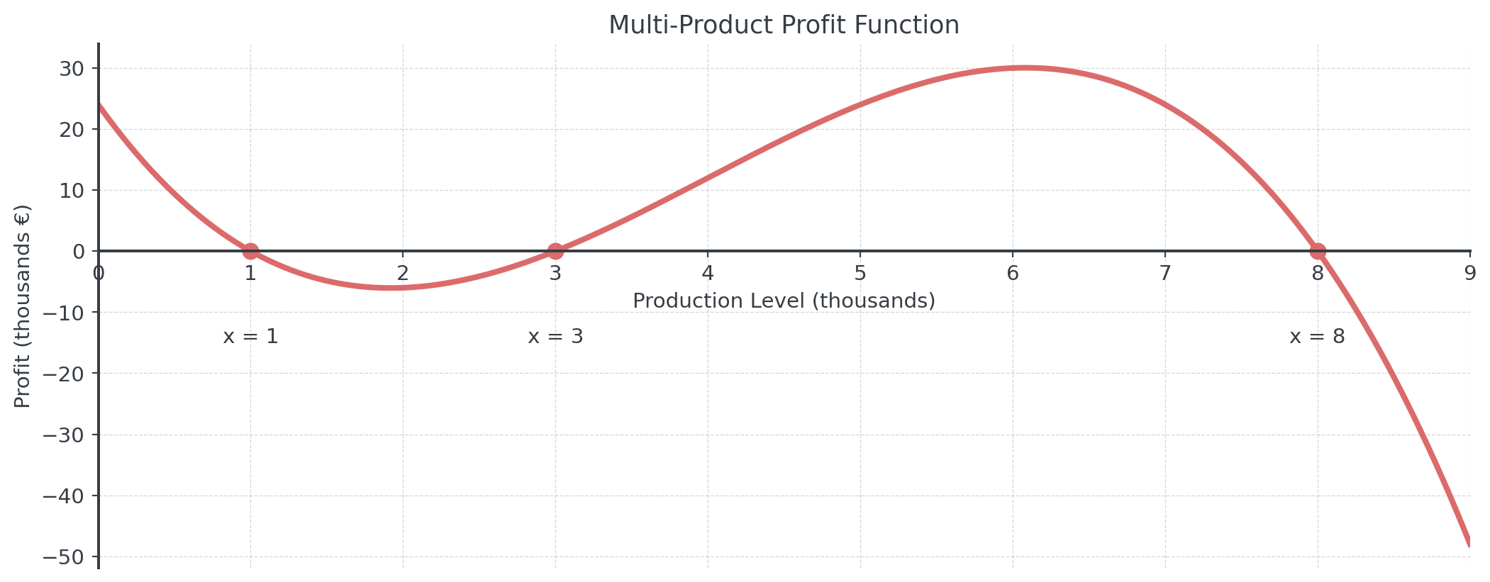
Analysis: Break-even at 1,000, 3,000, and 8,000 units
Cost Function with Scale Effects
Complex cost structures
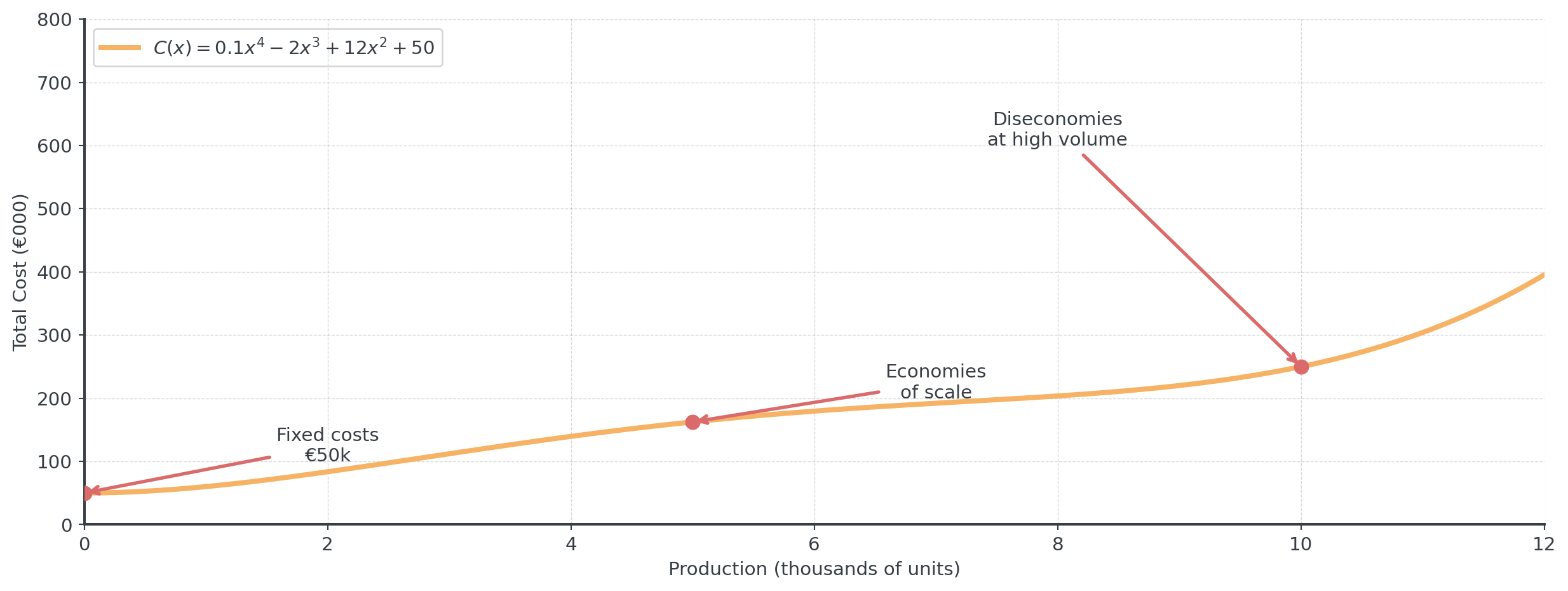
A manufacturing plant has cost function:
\[C(x) = 0.1x^4 - 2x^3 + 12x^2 + 50\]
- Fixed costs of €50,000 and variable costs
- Economies of scale (negative cubic)
- Diseconomies at high volume (positive quartic)
. . .
Polynomial cost functions capture the reality that unit costs often decrease initially (economies of scale) but may increase at very high production levels (capacity constraints).
Visualizing the Cost Function
Market Share Dynamics II
Problem-Solving - 30 Minutes
TechCo Case Study - Part II
TechCo needs your help with additional questions:
End Behavior Analysis: Their competitor has profit function \(C(x) = -3x^5 + 2x^4 - 7x^2 + x - 9\). Describe the long-term behavior as production increases. What does this tell management?
Product Line Analysis: A subsidiary’s profit is modeled by \(S(x) = 2(x + 2)^2(x - 3)(x - 5)^3\). Find all break-even points and describe how the company enters/exits profitability at each point.
New Product Launch: TechCo’s profit (in thousands €) for a new product after \(x\) months is: \(P(x) = -x^3 + 9x^2 - 15x - 25\). What is the initial financial position at launch and how is the profit at months 5 and 7?
Spot the Error
Can you find the errors? Work with your neighbor
Time allocation: 5 minutes to find errors, 5 minutes to discuss
Student work:
“The polynomial \(P(x) = 3x^4 - 2x^2 + 1\) has degree 2 because there are two terms with \(x\)”
“If \((x - 2)^4\) is a factor, the graph crosses the x-axis at \(x = 2\)”
“A degree 5 polynomial always has 5 real zeros”
Wrap-Up
Key Takeaways
Today’s essential concepts
- Polynomials extend our function toolkit to more complex scenarios
- Degree and leading coefficient tell the big picture story
- Zeros and multiplicities reveal detailed behavior
- Business applications involve multiple equilibrium points
- Mathematical tools prove what’s possible in business
Final Assessment
5 minutes - Individual work
Given the polynomial \(P(x) = -2x^3 + 6x^2 + 8x\):
Factor completely and find all zeros with their multiplicities
Determine the end behavior
Describe the graph’s behavior at each zero
If this represents a company’s profit (in thousands €) where \(x\) is production in thousands of units, at what production levels does the company break even?
Next Session Preview
Session 04-02: Power Functions & Roots
Building on polynomial foundations
- Power functions with rational exponents
- Root functions and their domains
- Transformations of power functions
- Economic models with diminishing returns
- Production functions in economics
. . .
Complete Tasks 04-01!