FSP Training 03

Preparation for Mock Exam 04

Instructions

This training page covers all of Section 03 and prepares you for Mock Exam 04. Set A trains setting up: you translate a text into mathematics and check your translation. Set B is a practice mock in the format of Mock Exam 04: 90 minutes, 50 points, and all 3 problems must be completed. Write down every step as you would in the exam. The points show what each part is worth.

In the real FSP, decimals are written with a comma (1,25 means 1.25).

Set A: Set Up & Check (40 minutes)

From Text to Mathematics (xx)

Translate each statement into mathematics. Then answer the check question: it tells you whether your translation works. (QU = quantity units, MU = monetary units)

1. “A bike-sharing provider charges \(B(t) = 1 + 0.15t\) EUR for a ride of \(t\) minutes. A customer asks: ‘How long can I ride for 10 EUR?’”

   Check: Does a ride of one hour cost at most 10 EUR?

2. “A clothing shop can sell \(x\) QU of rain jackets per month if it asks the price \(p(x) = 36 - 1.5x\) MU per QU (1 QU = 100 jackets, 1 MU = 100 EUR). Quantities and prices cannot be negative.” Give the domain and the range of \(p\) in this context.

   Check: Can the shop sell 2,500 rain jackets per month?

3. “A trampoline park counts its visitors. At an entrance price of 12 EUR, 330 people come per day, and at 15 EUR, 240 people come. The demand is linear.” Give the demand function \(Q_d(p)\) and the maximum price.

   Check: Do 150 people come at a price of 18 EUR?

4. “A manufactory bottles hot sauce. Its weekly total costs are \(C(x) = 2.4x + 35\) MU for \(x\) QU (1 QU = 1,000 bottles, 1 MU = 100 EUR). The variable costs per bottle are … EUR, and the fixed costs are … EUR per week.”

   Check: Do 5,000 bottles cause variable costs of 1,200 EUR?

5. An FSP task shows the graph of a quadratic function \(f\). The highest point of the graph is \((5, 32)\), and the graph crosses the \(x\)-axis at \(x = 1\). The task says: “Determine the function term of \(f\) in vertex form.” Give \(f(x)\).

   Check: Because of the symmetry, the graph crosses the \(x\)-axis a second time. Where? Does your term give 0 there?

6. “A muesli producer makes a weekly profit of \(P(x) = -x^2 + 16x - 39\) (in 1,000 EUR) with \(x\) tonnes of muesli. It can produce at most 14 tonnes per week.” Give the domain and the range of \(P\) in this context.

   Hint: A parabola that opens downward rises up to its vertex and falls after it, so on an interval its lowest value lies at one of the two ends.

   Check: A trainee computes \(P(0) = -39\) and \(P(14) = -11\) and says: “The producer always makes a loss.” Is the trainee right?

7. “The dairy farms of a region offer \(Q_s(p) = 5000p - 2000\) litres of organic milk per day at a price of \(p\) EUR per litre. The state now pays a subsidy of 0.10 EUR per litre: for each litre sold at the price \(p\), a farm receives \(p + 0.10\) EUR.” Give the new supply function and name the transformation.

   Check: At a price of 0.60 EUR per litre, do the farms now offer 500 litres more per day than before?

8. “A game studio’s new game is downloaded \(d(t) = -(t - 6)^2 + 36\) thousand times in week \(t\) after the launch (\(0 \leq t \leq 12\)). The studio expects its next game to be downloaded over a period twice as long, with the same highest number of downloads per week.” Give the function \(d_1(t)\) for the next game and name the transformation.

   Check: In which week does the next game reach its highest number of downloads, and after how many weeks do its downloads end?

9. “A small online shop sells wooden cutting boards. At a price of \(p(x) = 18 - 0.04x\) EUR per board, the customers buy \(x\) boards per month. The monthly costs are \(C(x) = 5x + 800\) EUR. The owner wants the costs as a function of the price.” Give the number of boards \(x(p)\) at the price \(p\) with its domain, and the composite function for the costs.

   Check: An assistant inserts a price of 20 EUR per board into your composite function. What does the assistant get, and why is the result meaningless?

CautionSolution

1. The 10 EUR are an amount of money, i.e. an output of \(B\). So the customer asks for the input \(t\) with \(B(t) = 10\):

   \[1 + 0.15t = 10 \iff 0.15t = 9 \iff t = 60\]

   Check: yes, \(B(60) = 1 + 9 = 10\) EUR. For 10 EUR, the customer can ride exactly one hour.

   Typical mistake: \(B(10) = 2.50\) EUR. This is the price of a ride of 10 minutes. The input of \(B\) is a time in minutes, not an amount of money.

2. Quantities cannot be negative, so \(x \geq 0\). Prices cannot be negative either:

   \[36 - 1.5x \geq 0 \iff 1.5x \leq 36 \iff x \leq 24\]

   Domain: \([0; 24]\). Each additional QU lowers the price, so \(p\) falls. The range lies between the values at the two ends, \(p(24) = 0\) and \(p(0) = 36\): range \([0; 36]\) MU per QU, i.e. from 0 EUR to 36 EUR per jacket.

   Check: no. 2,500 jackets are 25 QU, outside the domain: \(p(25) = 36 - 37.5 = -1.5 < 0\). Even at a price of 0 EUR, the customers take only 2,400 jackets per month (the market saturation).

   Typical mistake: swapping domain and range, e.g. the domain \([0; 36]\). The domain holds the inputs (quantities in QU), the range the outputs (prices in MU per QU).

3. The demand falls by \(330 - 240 = 90\) people when the price rises by \(15 - 12 = 3\) EUR:

   \[m = \frac{240 - 330}{15 - 12} = \frac{-90}{3} = -30 \text{ people per EUR}\]

   Point-slope form with \((12, 330)\): \(Q_d - 330 = -30(p - 12) \iff Q_d(p) = 690 - 30p\).

   Maximum price: \(690 - 30p = 0 \iff p = 23\) EUR. At 23 EUR or more, nobody comes, so \(Q_d(p)\) holds for \(0 \leq p \leq 23\).

   Check: yes, \(Q_d(18) = 690 - 540 = 150\) people.

   Typical mistake: the slope \(\frac{15 - 12}{240 - 330} = -\frac{1}{30}\), with the prices on top. The demand function has the price as its input, so the change in the number of people goes on top: people per EUR.

4. 1 MU per QU is 100 EUR per 1,000 bottles. So 2.4 MU per QU are 240 EUR per 1,000 bottles: the variable costs are 0.24 EUR per bottle. The fixed costs are \(C(0) = 35\) MU \(=\) 3,500 EUR per week.

   Check: yes. 5,000 bottles are 5 QU with variable costs of \(2.4 \cdot 5 = 12\) MU \(= 1{,}200\) EUR, and indeed \(5000 \cdot 0.24 = 1200\).

   Typical mistake: reading the coefficients as EUR and bottles: 2.40 EUR per bottle and 35 EUR of fixed costs. Then 5,000 bottles would cause variable costs of 12,000 EUR. Convert MU and QU before you interpret a number.

5. Vertex form \(f(x) = a(x - h)^2 + k\) with the vertex \((h, k) = (5, 32)\): \(f(x) = a(x - 5)^2 + 32\). Insert the zero \(x = 1\):

   \[0 = a(1 - 5)^2 + 32 = 16a + 32 \iff a = -2 \qquad \Rightarrow \qquad f(x) = -2(x - 5)^2 + 32\]

   Check: the axis of symmetry is \(x = 5\). The zero \(x = 1\) lies 4 units to the left of it, so the second zero lies 4 units to the right of it, at \(x = 9\): \(f(9) = -2 \cdot 16 + 32 = 0\) ✓

   Typical mistake: \(f(x) = a(x + 5)^2 + 32\). This parabola has its vertex at \(x = -5\). With the zero \(x = 1\) it gives \(36a + 32 = 0\), i.e. \(a = -\frac{8}{9}\), and then \(f(9) \neq 0\). The vertex \((h, k)\) belongs to \((x - h)^2\), so \(h = 5\) gives \((x - 5)^2\).

6. Domain: \([0; 14]\). \(P\) is a parabola that opens downward (\(a = -1 < 0\)), so its vertex is a maximum:

   \[x_v = -\frac{16}{2 \cdot (-1)} = 8, \qquad P(8) = -64 + 128 - 39 = 25\]

   The vertex lies in the domain. Left of the axis of symmetry \(x = 8\) the profit rises, right of it the profit falls. So the smallest value lies at one of the two ends: \(P(0) = -39\) and \(P(14) = -196 + 224 - 39 = -11\). Range: \([-39; 25]\), i.e. from a loss of 39,000 EUR to a profit of 25,000 EUR per week.

   Check: no. With 8 tonnes, the producer makes its highest profit, 25,000 EUR per week.

   Typical mistake: taking only the values at the two ends of the domain. This only works for a function that grows or falls on the whole domain. A parabola with its vertex inside the domain turns around at the vertex.

7. A farm offers according to the amount it receives, \(p + 0.10\) EUR per litre. So the input \(p\) is replaced by \(p + 0.10\):

   \[Q_{s,\text{new}}(p) = Q_s(p + 0.10) = 5000(p + 0.10) - 2000 = 5000p - 1500\]

   This is a horizontal shift by 0.10 to the left.

   Check: yes. \(Q_s(0.60) = 3000 - 2000 = 1000\) litres and \(Q_{s,\text{new}}(0.60) = 3000 - 1500 = 1500\) litres, i.e. 500 litres more per day. The supply now starts at a price of 0.30 EUR per litre instead of 0.40 EUR.

   Typical mistake: \(Q_s(p - 0.10) = 5000p - 2500\). This shifts the graph to the right, as a tax would do, and the farms would offer 500 litres less despite the subsidy. Plus shifts left, minus shifts right.

8. Every phase of the downloads takes twice as long, so the cycle runs half as fast. A horizontal stretch by the factor \(b = 2\) replaces \(t\) by \(\frac{t}{2}\) (rule \(g(x) = f\left(\frac{x}{b}\right)\) with \(b > 1\)), as in the product lifecycle example of the lecture:

   \[d_1(t) = -\left(\frac{t}{2} - 6\right)^2 + 36 = -\frac{1}{4}(t - 12)^2 + 36, \qquad 0 \leq t \leq 24\]

   This is a horizontal stretch by the factor 2.

   Check: the next game reaches its highest number of downloads, 36,000, in week 12, and its downloads end after 24 weeks (the first game: week 6 and 12 weeks).

   Typical mistake: \(d(2t) = -(2t - 6)^2 + 36 = -4(t - 3)^2 + 36\). This is a horizontal compression: the peak would come in week 3, and the downloads would end after 6 weeks. \(f(2t)\) compresses (faster), \(f\left(\frac{t}{2}\right)\) stretches (slower).

9. Number of boards: solve \(p = 18 - 0.04x\) for \(x\):

   \[0.04x = 18 - p \iff x(p) = 450 - 25p\]

   The number of boards cannot be negative: \(450 - 25p \geq 0 \iff p \leq 18\). Domain: \(0 \leq p \leq 18\) (18 EUR is the maximum price).

   Costs as a function of the price: first \(x(p)\) gives the number of boards, then \(C\) gives the costs for this number:

   \[(C \circ x)(p) = C(450 - 25p) = 5(450 - 25p) + 800 = 3050 - 125p, \qquad 0 \leq p \leq 18\]

   Check: the assistant gets \(3050 - 2500 = 550\) EUR. This is less than the fixed costs of 800 EUR, so it cannot be the costs. The reason: \(x(20) = 450 - 500 = -50\) boards, a negative number. 20 EUR lies above the maximum price and outside the domain. At 20 EUR nobody buys a board, and the costs are the fixed costs, \(C(0) = 800\) EUR.

   Typical mistake: using the composite term for every price. A composite function is only defined where the inner function delivers an allowed input for the outer function, here \(x(p) \geq 0\).

One Paragraph, All Conditions (xx)

A company builds portable power stations (large batteries for camping and for power cuts) and sells them to electronics stores. The stores buy no power station at a price of 960 EUR or more (maximum price). At a price of 0 EUR, they would take 3,200 power stations per month (market saturation). In between, the demand is linear. The fixed costs are 140,000 EUR per month, and each power station costs 330 EUR for battery cells and assembly. The factory can build at most 2,000 power stations per month (capacity). The owner wants to know the output with the highest profit, the price for this output, and how many power stations the stores buy at a price of 720 EUR. From next year on, a new safety test will add 30 EUR to the costs of every power station.

(1 QU = 100 power stations, 1 MU = 1,000 EUR, so a price of \(p\) MU per QU is a price of \(10p\) EUR per power station)

List the price-demand function \(p(x)\) in MU per QU, the revenue \(R(x)\), the total costs \(C(x)\) and the profit \(P(x)\) in MU, the domain of \(x\) in this context, a condition or formula for each of the owner’s three questions, and the total costs \(C_1(x)\) after the safety test. Do not solve anything.

Check: A trainee writes the new total costs as \(C(x) + 30\). Compare the additional costs for 2,000 power stations with the trainee’s term and with yours.

CautionSolution

1. Price-demand function: 960 EUR per power station \(= 96\) MU per QU, and 3,200 power stations \(= 32\) QU. From \(p(0) = 96\) and \(p(32) = 0\), the slope is \(-\frac{96}{32} = -3\): \(p(x) = 96 - 3x\)
2. Revenue: \(R(x) = x \cdot p(x) = 96x - 3x^2\)
3. Total costs: 140,000 EUR \(= 140\) MU, and 330 EUR per power station \(= 33{,}000\) EUR per QU \(= 33\) MU per QU: \(C(x) = 33x + 140\)
4. Profit: \(P(x) = R(x) - C(x) = -3x^2 + 63x - 140\)
5. Domain: \(0 \leq x \leq 20\) (the capacity of 2,000 power stations lies below the market saturation)
6. Highest profit: \(x_v = -\frac{63}{2 \cdot (-3)}\), a maximum since \(a = -3 < 0\). It is only allowed if \(x_v \leq 20\)
7. Price for this output: \(p(x_v)\) in MU per QU, times 10 for EUR per power station
8. At 720 EUR per power station \(= 72\) MU per QU: \(96 - 3x = 72\), or the inverse function \(x(p) = 32 - \frac{p}{3}\) and \(x(72)\)
9. After the safety test: 30 EUR per power station \(= 3{,}000\) EUR per QU \(= 3\) MU per QU more, so \(C_1(x) = 36x + 140\)

Check: 2,000 power stations are 20 QU. With your term, the additional costs are \(C_1(20) - C(20) = 3 \cdot 20 = 60\) MU \(= 60{,}000\) EUR, i.e. 30 EUR for each of the 2,000 power stations. The trainee’s term adds only 30 MU \(= 30{,}000\) EUR, and the same amount at every output, like a fixed cost.

Typical mistake: \(C(x) + 30\), a vertical shift. A cost per unit changes the variable costs per QU (the slope of \(C\)), not the fixed costs. And 30 EUR per power station are 3 MU per QU, not 30 MU.

FSP Words So Far

The FSP problems use these words from Sections 01 to 03. Learn what each one means and how to write it in mathematics.

Word	Meaning	Mathematics
quantity unit (QU)	a fixed number of items, e.g. 1 QU = 100 items	the output \(x\) is counted in QU
monetary unit (MU)	a fixed amount of money, e.g. 1 MU = 100 EUR	results in MU, convert to EUR at the end
fixed costs	costs that arise even if nothing is produced	the constant term of \(C(x)\)
variable costs	costs that grow with the output	output times costs per QU
total costs	fixed costs + variable costs	\(C(x)\)
revenue	quantity times price	\(R(x) = x \cdot \text{price}\)
profit	revenue − total costs	\(P(x) = R(x) - C(x)\)
break-even point	the output at which the profit changes from negative (a loss) to positive	\(P(x) = 0\), the smaller zero
profit limit (upper break-even point)	the larger output with zero profit: above it, the profit turns negative again	\(P(x) = 0\), the larger zero
profit zone	all outputs with a positive profit	\(P(x) > 0\): from the break-even point to the profit limit (or the capacity)
capacity	the maximum possible output	an upper bound: \(x \leq\) capacity
growth factor	the factor by which a quantity is multiplied each period	\(q\) in (starting value) \(\cdot\, q^t\)
growth rate	the change per period in percent	\(q = 1 + r\) with \(r\) as a decimal, a loss of 4 % gives \(q = 0.96\)
doubling time	the time after which a quantity has doubled	\(q^T = 2\)
half-life (halving time)	the time after which a quantity has halved	\(q^T = 0.5\)
“deviates from \(a\) by at most \(d\)” (tolerance)	the distance from \(a\) is at most \(d\)	\(\lvert x - a \rvert \leq d \iff a - d \leq x \leq a + d\)
“share of \(A\) among \(B\)”	the part of \(B\) that also belongs to \(A\): the base is \(B\)	\(\dfrac{\text{number in } A \cap B}{\text{number in } B}\)
“neither \(A\) nor \(B\)”	not in \(A\) and not in \(B\), i.e. outside both circles	\(\overline{A \cup B}\)
contingency table	a table of counts for two properties: the inner fields are the regions of the Venn diagram, the margins are the totals	inner fields \(A \cap B\), \(A \cap \overline{B}\), \(\overline{A} \cap B\), \(\overline{A} \cap \overline{B}\)
gross price, net price	gross price = net price + VAT	with 19 % VAT: gross \(= 1.19 \cdot\) net
system of linear equations	several linear equations that must hold at the same time	solve by substitution or elimination, check the solution in every equation
no solution, infinitely many solutions	the conditions contradict each other, or one condition only repeats another	elimination leaves \(0 = d\) with \(d \neq 0\), or \(0 = 0\)
demand, supply	the quantity buyers want to buy and the quantity sellers offer at a given price	as terms in the price \(p\), e.g. \(Q_d(p)\), \(Q_s(p)\), or as prices \(p_D(x)\), \(p_S(x)\) for the quantity \(x\)
market equilibrium	the quantity demanded equals the quantity supplied	demand = supply: \(Q_d(p) = Q_s(p)\), or \(p_D(x) = p_S(x)\)
price-demand function	gives the price at which \(x\) QU can be sold	\(p(x)\), revenue \(R(x) = x \cdot p(x)\)
average cost	total costs divided by the number of units	\(\dfrac{C(x)}{x}\) with \(x \neq 0\)
zero form	all terms on one side, 0 on the other side	\(ax^2 + bx + c = 0\), then factor or use the quadratic formula
discriminant	decides how many real solutions a quadratic equation has	\(\Delta = b^2 - 4ac\): \(> 0\) two, \(= 0\) one, \(< 0\) none
biquadratic equation	an equation with only \(x^4\), \(x^2\) and a constant	substitute \(u = x^2\) in \(ax^4 + bx^2 + c\), solve for \(u\), then \(x = \pm\sqrt{u}\) for \(u \geq 0\)
domain restrictions (of an equation)	the conditions the unknown must meet so that every term is defined	denominators \(\neq 0\), under a root \(\geq 0\), inside a logarithm \(> 0\)
extraneous solution	a candidate that solves the squared equation but not the original one	check every candidate in the original equation
function	assigns to every input exactly one output	\(f(x)\), its graph passes the vertical line test
domain (of a function)	all inputs for which the function is defined, in a context only the sensible ones	e.g. \([0; \text{capacity}]\)
range	all outputs that the function takes on its domain	if the function grows or falls: between the values at the two ends, for a parabola also check the vertex
maximum price	the price at which nobody buys any more	\(Q_d(p) = 0\), or \(c\) in \(p = c - dQ\)
market saturation	the quantity demanded at a price of 0	\(a\) in \(Q_d = a - bp\), or the zero of \(p(x)\)
shortage, surplus	at a price below the equilibrium price, demand exceeds supply (shortage), above it, supply exceeds demand (surplus)	\(Q_d(p) > Q_s(p)\), or \(Q_d(p) < Q_s(p)\)
contribution margin	price minus variable costs per unit: the part of the price that covers the fixed costs	break-even quantity \(= \dfrac{\text{fixed costs}}{\text{contribution margin}}\)
vertex	the highest or lowest point of a parabola	\(x_v = -\dfrac{b}{2a}\), or \((h, k)\) in \(a(x - h)^2 + k\)
profit-maximizing output	the output with the highest profit	\(x_v\) of \(P(x)\), a maximum since \(a < 0\), and the price \(p(x_v)\). If the capacity lies below \(x_v\): the capacity and its price
shift, stretch, compression	moving or scaling a graph	\(a \cdot f(b(x - h)) + k\): first \(b\), then \(h\), then \(a\), then \(k\)
mirror image at the \(y\)-axis	the graph flipped from right to left	\(f(-x)\)
mirror image at the \(x\)-axis	the graph flipped upside down	\(-f(x)\)
composite function	first the inner function, then the outer function	\((f \circ g)(x) = f(g(x))\)
inverse function	reverses a function: gives the input that belongs to an output	solve \(y = f(x)\) for \(x\), e.g. \(x(p)\) from \(p(x)\)

In set-builder notation, \(\{x \in \mathbb{R} \mid \dots\}\) and \(\{x \in \mathbb{R} : \dots\}\) mean the same.

Set B: Practice Mock (90 minutes, 50 points)

Problem 1: Air Purifiers [20 pts. total]

A company builds air purifiers for offices and schools. Its fixed costs (rent, staff, development) amount to 320,000 EUR per month. For an output of \(x\) QU per month, it models its variable costs (they grow with the output) by \((1.5x^2 + 12x)\) MU: the larger the output, the more each additional air purifier costs, because the staff then work night shifts with a wage bonus and the scarce filter material becomes more expensive.

(QU = quantity units, MU = monetary units. 1 QU = 100 air purifiers, 1 MU = 1,000 EUR, so a price of \(p\) MU per QU is a price of \(10p\) EUR per air purifier. Total costs = fixed costs + variable costs. Revenue = quantity × price. Profit = revenue − total costs.)

1. Determine the linear price-demand function \(p(x)\) (price in MU per QU at a demand of \(x\) QU per month) assuming a maximum price of 920 EUR per air purifier and a market saturation at 9,200 air purifiers per month. Give terms for the revenue function \(R(x)\) and the cost function \(C(x)\).

(for verification: \(p(x) = 92 - x\))

[4 pts.]

2. Show that the profit function is given by \(P(x) = -2.5x^2 + 80x - 320\).

[2 pts.]

3. Determine the (lower) break-even point and the profit limit (upper break-even point) with the quadratic formula, exactly and in QU rounded to two decimal places. Decide in which output range the company makes a profit and give the smallest and the largest number of air purifiers per month with which it makes a profit.

[4 pts.]

4. Compute the maximum profit in EUR and prove that it really is a maximum. Calculate the price per air purifier in EUR that the company must ask to sell exactly the profit-maximizing output.

[4 pts.]

5. Calculate the number of sold air purifiers and the profit in EUR if the company asks for a price of 820 EUR per air purifier. Compare the profit with d).

[3 pts.]

6. This year, the filter supplier can only deliver filters for at most 1,400 air purifiers per month. Determine the output with the highest profit under this restriction and give a reason. Calculate the price per air purifier the company should now ask and the monthly profit in EUR.

Hint: A parabola that opens downward rises up to its vertex and falls after it. If the whole domain lies left of the vertex, the largest value lies at the right end of the domain.

[3 pts.]

CautionSolutions

a) Units. A price of 920 EUR per air purifier means \(100 \cdot 920 = 92{,}000\) EUR \(= 92\) MU per QU. The market saturation is 9,200 air purifiers \(= 92\) QU.

Linear price-demand function \(p(x) = c - dx\). At the maximum price the demand is 0, so \(p(0) = 92\) and \(c = 92\). At the market saturation the price is 0:

\[p(92) = 92 - 92d = 0 \iff d = 1 \qquad \Rightarrow \qquad p(x) = 92 - x, \quad 0 \leq x \leq 92\]

Revenue = quantity × price:

\[R(x) = x \cdot p(x) = x(92 - x) = -x^2 + 92x\]

Costs. Fixed costs 320,000 EUR \(= 320\) MU. Total costs = fixed costs + variable costs:

\[C(x) = 1.5x^2 + 12x + 320\]

Grading: 1 Pt. conversion of maximum price and market saturation to MU per QU and QU, 1 Pt. \(p(x)\), 1 Pt. \(R(x) = x \cdot p(x)\), 1 Pt. \(C(x)\) with the fixed costs in MU.

b)

\[P(x) = R(x) - C(x) = (-x^2 + 92x) - (1.5x^2 + 12x + 320)\]

The minus sign changes every sign in the second bracket:

\[P(x) = -x^2 + 92x - 1.5x^2 - 12x - 320 = -2.5x^2 + 80x - 320 \quad \checkmark\]

Grading: 1 Pt. ansatz \(P = R - C\), 1 Pt. sign change and collecting terms.

c) Zero form. At a break-even point the profit is zero, \(P(x) = 0\). Divide by \(-2.5\):

\[-2.5x^2 + 80x - 320 = 0 \;\big|: (-2.5) \iff x^2 - 32x + 128 = 0\]

Quadratic formula with \(\Delta = (-32)^2 - 4 \cdot 1 \cdot 128 = 1024 - 512 = 512\) and \(\sqrt{512} = \sqrt{256 \cdot 2} = 16\sqrt{2}\):

\[x_{1,2} = \frac{32 \pm 16\sqrt{2}}{2} = 16 \pm 8\sqrt{2}, \qquad x_1 \approx 4.69, \qquad x_2 \approx 27.31\]

Both zeros lie in the domain \([0; 92]\). Break-even point: \(x_1 = 16 - 8\sqrt{2} \approx 4.69\) QU. Profit limit: \(x_2 = 16 + 8\sqrt{2} \approx 27.31\) QU.

Profit zone. The parabola opens downward (\(a = -2.5 < 0\)), so the profit is positive between the zeros. Test value: \(P(16) = -640 + 1280 - 320 = 320 > 0\) ✓. Profit zone: \((16 - 8\sqrt{2}; 16 + 8\sqrt{2}) \approx (4.69; 27.31)\).

Whole air purifiers. \(x_1 \approx 4.6863\) QU \(= 468.63\) air purifiers and \(x_2 \approx 27.3137\) QU \(= 2731.37\) air purifiers. Round the lower bound up and the upper bound down: the company makes a profit with 469 to 2,731 air purifiers per month.

Check: 468 air purifiers give \(P(4.68) = -54.756 + 374.4 - 320 \approx -0.36\) MU, a loss of about 360 EUR.

Grading: 1 Pt. zero form, 1 Pt. quadratic formula with discriminant, 1 Pt. exact and rounded values named as break-even point and profit limit, 1 Pt. profit zone with reason and 469 to 2,731 air purifiers.

d) Vertex formula:

\[x_v = -\frac{80}{2 \cdot (-2.5)} = 16 \text{ QU} = 1{,}600 \text{ air purifiers per month}\]

(The vertex lies halfway between the zeros \(16 - 8\sqrt{2}\) and \(16 + 8\sqrt{2}\) ✓.)

Maximum profit:

\[P(16) = -2.5 \cdot 256 + 80 \cdot 16 - 320 = -640 + 1280 - 320 = 320 \text{ MU} = 320{,}000 \text{ EUR per month}\]

Proof. \(a = -2.5 < 0\), the parabola opens downward, so the vertex is a maximum.

Price: \(p(16) = 92 - 16 = 76\) MU per QU \(= 10 \cdot 76 = 760\) EUR per air purifier.

Grading: 1 Pt. \(x_v = 16\), 1 Pt. maximum profit of 320,000 EUR, 1 Pt. proof with \(a < 0\), 1 Pt. price of 760 EUR per air purifier.

e) Units. 820 EUR per air purifier \(= 82\) MU per QU. The price-demand function gives the quantity:

\[92 - x = 82 \iff x = 10 \text{ QU} = 1{,}000 \text{ air purifiers per month}\]

Profit:

\[P(10) = -2.5 \cdot 100 + 80 \cdot 10 - 320 = -250 + 800 - 320 = 230 \text{ MU} = 230{,}000 \text{ EUR}\]

This is 90,000 EUR less than the maximum profit from d). At 820 EUR, the price is too high: the company sells only 1,000 instead of 1,600 air purifiers.

Grading: 1 Pt. conversion and equation \(p(x) = 82\), 1 Pt. 1,000 air purifiers, 1 Pt. profit of 230,000 EUR with the comparison.

f) Now \(0 \leq x \leq 14\), and the vertex \(x_v = 16\) lies outside this domain. Since \(a = -2.5 < 0\), the parabola opens downward. Left of its axis of symmetry \(x = 16\), the profit rises towards the vertex, and the whole domain \([0; 14]\) lies left of it. So the highest allowed profit lies at the edge closest to the vertex: 1,400 air purifiers per month. Test value: \(P(13) = -422.5 + 1040 - 320 = 297.5 < P(14)\) ✓

Price: to sell exactly 1,400 air purifiers, the company asks \(p(14) = 92 - 14 = 78\) MU per QU, i.e. 780 EUR per air purifier. At the price of 760 EUR from d), the customers would want 1,600 air purifiers, but only 1,400 can be built.

Profit:

\[P(14) = -2.5 \cdot 196 + 80 \cdot 14 - 320 = -490 + 1120 - 320 = 310 \text{ MU} = 310{,}000 \text{ EUR per month}\]

That is 10,000 EUR less than without the restriction.

Grading: 1 Pt. 1,400 air purifiers with reason (\(a < 0\), axis of symmetry, test value), 1 Pt. price of 780 EUR, 1 Pt. profit of 310,000 EUR.

Problem 2: A Parabola and Its Mirror Images [17 pts. total]

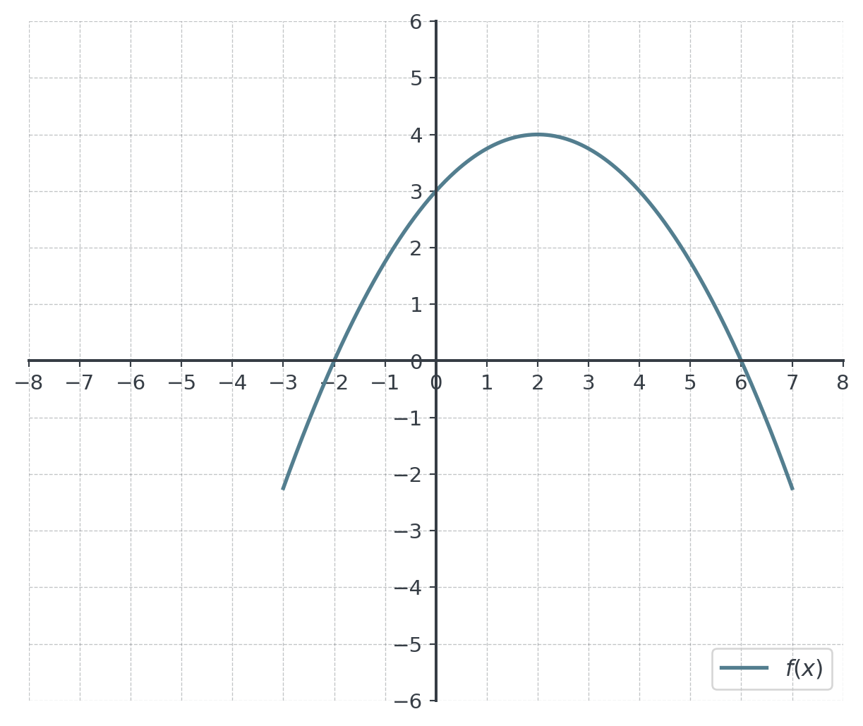
The figure shows the graph of a quadratic function \(f\).

Figure 1: Graph of the quadratic function f

1. Determine the function term of \(f\) in factored form and in standard form. Use information obtained from the graph.

(for verification: \(f(x) = -0.25x^2 + x + 3\))

[3 pts.]

2. Determine the vertex of \(f\) by calculation and give \(f\) in vertex form. Give the range of \(f\).

[3 pts.]

3. Give a function \(f_1(x)\) which is a mirror image of \(f(x)\) mirrored at the \(y\)-axis and give a reason for your choice. Graph \(f_1\) directly into the figure.

[4 pts.]

4. Determine computationally all points at which the graphs of \(f\) and \(f_1\) intersect. Explain why the graph of a function and its mirror image at the \(y\)-axis always have the point \((0, f(0))\) in common.

[2 pts.]

5. The graph of \(f\) is first shifted 2 units to the left, then compressed vertically by the factor 0.5 and mirrored at the \(x\)-axis, and finally shifted 3 units down. This gives the graph of a function \(g\). Give a term for \(g(x)\) in terms of \(f\) and show that \(g(x) = 0.125x^2 - 5\). Explain why the graph of \(g\) is its own mirror image at the \(y\)-axis.

[3 pts.]

6. Determine the zeros of \(g\) exactly. A student does the last two steps of e) in the other order: first the shift 3 units down, then the compression by 0.5 and the mirror image at the \(x\)-axis. Determine the zeros of the student’s function and explain the difference.

[2 pts.]

CautionSolutions

a) Read off: the graph crosses the \(x\)-axis at \(x = -2\) and \(x = 6\) and the \(y\)-axis at \((0, 3)\).

Factored form with the zeros: \(f(x) = a(x + 2)(x - 6)\). Insert the \(y\)-intercept \((0, 3)\):

\[3 = a \cdot 2 \cdot (-6) = -12a \iff a = -0.25\]

\[f(x) = -0.25(x + 2)(x - 6)\]

Standard form:

\[f(x) = -0.25(x^2 - 4x - 12) = -0.25x^2 + x + 3 \quad \checkmark\]

Check with a further point of the graph: \(f(2) = -1 + 2 + 3 = 4\), and the graph passes through \((2, 4)\) ✓

Grading: 1 Pt. zeros and ansatz in factored form, 1 Pt. \(a = -0.25\) from the \(y\)-intercept, 1 Pt. standard form.

b) Vertex formula: \(x_v = -\frac{1}{2 \cdot (-0.25)} = 2\) and \(f(2) = 4\). The vertex is \((2, 4)\). It lies halfway between the zeros \(-2\) and \(6\) ✓

Vertex form: \(f(x) = -0.25(x - 2)^2 + 4\). Check: \(-0.25(x^2 - 4x + 4) + 4 = -0.25x^2 + x + 3\) ✓

Range: \(a = -0.25 < 0\), the parabola opens downward, so the vertex is its highest point. The values fall without bound the further \(x\) moves away from 2. Range: \((-\infty; 4]\).

Grading: 1 Pt. vertex, 1 Pt. vertex form, 1 Pt. range with reason.

c) Replace \(x\) by \(-x\):

\[f_1(x) = f(-x) = -0.25(-x)^2 + (-x) + 3 = -0.25x^2 - x + 3 = -0.25(x + 2)^2 + 4\]

Reason: replacing \(x\) by \(-x\) maps each point \((a, f(a))\) of the graph of \(f\) to the point \((-a, f(a))\). Every point keeps its height and moves to the other side of the \(y\)-axis at the same distance, so the graph is mirrored at the \(y\)-axis.

Graph: vertex \((-2, 4)\), zeros \(x = -6\) and \(x = 2\) (the mirror images of \(6\) and \(-2\)), \(y\)-intercept \((0, 3)\).

Figure 2: The graphs of f and of its mirror image f₁

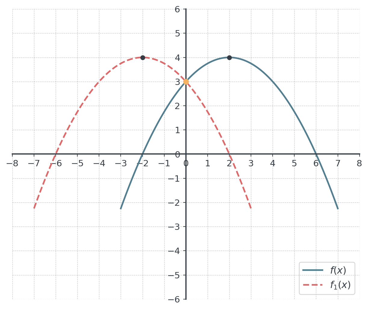
Grading: 1 Pt. \(f_1(x) = f(-x)\) simplified, 1 Pt. reason, 2 Pts. graph (vertex, zeros, \(y\)-intercept).

d) Set the two terms equal:

\[-0.25x^2 + x + 3 = -0.25x^2 - x + 3 \iff x = -x \iff 2x = 0 \iff x = 0\]

\(f(0) = 3\), so the only intersection point is \(S(0, 3)\), on the \(y\)-axis.

Explanation: at \(x = 0\), the mirror image has the value \(f_1(0) = f(-0) = f(0)\). The point on the \(y\)-axis is its own mirror image, so both graphs pass through \((0, f(0))\).

Grading: 1 Pt. equation and intersection point \((0, 3)\), 1 Pt. explanation.

e) Order as in \(a \cdot f(b(x - h)) + k\): shift to the left by 2 (\(x + 2\)), then the factor \(-0.5\) (compression by 0.5 and mirror image at the \(x\)-axis), and the shift down by 3 last:

\[g(x) = -0.5 \cdot f(x + 2) - 3\]

With the vertex form from b): \(f(x + 2) = -0.25\big((x + 2) - 2\big)^2 + 4 = -0.25x^2 + 4\), so

\[g(x) = -0.5\left(-0.25x^2 + 4\right) - 3 = 0.125x^2 - 2 - 3 = 0.125x^2 - 5 \quad \checkmark\]

Own mirror image: \(g(-x) = 0.125(-x)^2 - 5 = 0.125x^2 - 5 = g(x)\). Mirroring \(g\) at the \(y\)-axis gives \(g\) again. The vertex \((0, -5)\) lies on the \(y\)-axis, so the \(y\)-axis is the axis of symmetry of the parabola.

Grading: 1 Pt. \(g(x) = -0.5 \cdot f(x + 2) - 3\), 1 Pt. simplification to \(0.125x^2 - 5\), 1 Pt. \(g(-x) = g(x)\) with reason.

f) Zeros of \(g\):

\[0.125x^2 - 5 = 0 \iff x^2 = 40 \iff x = \pm\sqrt{40} = \pm 2\sqrt{10} \approx \pm 6.32\]

Student’s function: the shift down comes before the factor \(-0.5\), so the factor also acts on the shift:

\[h(x) = -0.5\big(f(x + 2) - 3\big) = -0.5\left(-0.25x^2 + 1\right) = 0.125x^2 - 0.5\]

\[0.125x^2 - 0.5 = 0 \iff x^2 = 4 \iff x = \pm 2\]

The factor \(-0.5\) turns the shift of 3 down into a shift of 1.5 up. The vertex lies at \((0, -0.5)\) instead of \((0, -5)\), so the zeros move closer together. The order of the steps matters.

Grading: 1 Pt. zeros \(\pm 2\sqrt{10}\), 1 Pt. zeros \(\pm 2\) of the student’s function with explanation.

Problem 3: Pumpkin Market [13 pts. total]

In autumn, farms sell pumpkins at the weekly farmers’ markets of a town. The customers’ demand is described by the price-demand function \(p_D(Q) = 6 - 0.002Q\): at a price of \(p_D(Q)\) EUR per kg, the customers buy \(Q\) kg of pumpkins per week. The farms together offer 400 kg per week at a price of 2.50 EUR per kg and 800 kg per week at a price of 3.50 EUR per kg. The supply is linear.

1. Give the demand as a function of the price, \(Q_d(p)\). Set up the supply function \(Q_s(p)\) with the point-slope form and determine the price below which the farms offer no pumpkins. Determine the market equilibrium.

(for verification: equilibrium price 4 EUR per kg)

[4 pts.]

2. Only prices from the price at which the supply starts up to the maximum price are relevant. Determine the inverse function \(p_S(Q)\) of the supply function and give its domain and range in this context. Explain its meaning and calculate the lowest price at which the farms offer 1,400 kg per week.

[3 pts.]

3. Farms from a neighbouring village join the markets. From now on, the farms together offer 25 % more pumpkins at every price. Give the new supply function and describe how its graph arises from the graph of \(Q_s\). Determine the new market equilibrium and interpret the change.

[3 pts.]

4. After the harvest, the farms sell their stored pumpkins. In week \(t\) after the end of the harvest, they bring \(H(t) = 1750 - 150t\) kg to the markets and set the price at which the customers buy exactly this quantity. Give a term for the composite function \((p_D \circ H)(t)\) and explain its meaning and the meaning of its slope. Determine from which week on the price is higher than 4 EUR per kg.

(for verification: \((p_D \circ H)(t) = 2.5 + 0.3t\))

[3 pts.]

CautionSolutions

a) Demand as a function of the price. Solve \(p = 6 - 0.002Q\) for \(Q\):

\[0.002Q = 6 - p \iff Q_d(p) = 3000 - 500p\]

Supply. Slope from the two points \((2.5, 400)\) and \((3.5, 800)\):

\[m = \frac{800 - 400}{3.5 - 2.5} = 400 \text{ kg per EUR}\]

Point-slope form with \((2.5, 400)\):

\[Q_s(p) - 400 = 400(p - 2.5) \iff Q_s(p) = 400p - 1000 + 400 = 400p - 600\]

Check: \(Q_s(3.5) = 1400 - 600 = 800\) ✓

No supply: \(400p - 600 = 0 \iff p = 1.5\). Below 1.50 EUR per kg, the farms offer no pumpkins.

Equilibrium: supply equals demand.

\[3000 - 500p = 400p - 600 \iff 3600 = 900p \iff p^* = 4\]

\[Q^* = Q_d(4) = 3000 - 2000 = 1000 \qquad \text{Check: } Q_s(4) = 1600 - 600 = 1000 \; \checkmark\]

At 4 EUR per kg, the customers buy exactly as many pumpkins as the farms offer: 1,000 kg per week.

Grading: 1 Pt. \(Q_d(p)\), 1 Pt. \(Q_s(p)\) and 1.50 EUR, 1 Pt. equation and equilibrium price, 1 Pt. equilibrium quantity with check.

b) Inverse function. Solve \(Q = 400p - 600\) for \(p\):

\[400p = Q + 600 \iff p_S(Q) = \frac{Q + 600}{400} = 1.5 + 0.0025Q\]

Domain and range. The relevant prices run from 1.50 EUR (start of the supply) to the maximum price \(p_D(0) = 6\) EUR. \(Q_s\) grows, so it takes the values from \(Q_s(1.5) = 0\) to \(Q_s(6) = 2400 - 600 = 1800\). For the inverse function, domain and range swap:

\[D = [0; 1800] \text{ kg}, \qquad W = [1.5; 6] \text{ EUR per kg}\]

Meaning: \(p_S(Q)\) gives the price at which the farms offer \(Q\) kg per week, i.e. the lowest price they need for this quantity. The intercept \(p_S(0) = 1.5\) is the price at which the supply starts.

1,400 kg: \(p_S(1400) = 1.5 + 3.5 = 5\) EUR per kg. Check: \(Q_s(5) = 2000 - 600 = 1400\) ✓

Grading: 1 Pt. inverse function, 1 Pt. domain and range, 1 Pt. meaning and 5 EUR per kg.

c) New supply: every supply value is multiplied by 1.25:

\[Q_{s,\text{new}}(p) = 1.25 \cdot Q_s(p) = 1.25(400p - 600) = 500p - 750\]

Graph: a vertical stretch of the graph of \(Q_s\) by the factor 1.25 (with \(p\) on the horizontal axis). The zero stays at \(p = 1.5\), since \(1.25 \cdot 0 = 0\): the supply still starts at 1.50 EUR per kg.

New equilibrium:

\[3000 - 500p = 500p - 750 \iff 3750 = 1000p \iff p^*_{\text{new}} = 3.75\]

\[Q^*_{\text{new}} = 3000 - 500 \cdot 3.75 = 1125 \qquad \text{Check: } Q_{s,\text{new}}(3.75) = 1875 - 750 = 1125 \; \checkmark\]

Interpretation: the larger supply lowers the equilibrium price by 0.25 EUR to 3.75 EUR per kg, and the customers buy 125 kg more per week, 1,125 kg. The customers gain from the new farms.

Grading: 1 Pt. new supply function with the vertical stretch, 1 Pt. new equilibrium, 1 Pt. interpretation.

d) First \(H\) gives the quantity in week \(t\), then \(p_D\) gives the price for this quantity:

\[(p_D \circ H)(t) = p_D(1750 - 150t) = 6 - 0.002(1750 - 150t) = 6 - 3.5 + 0.3t = 2.5 + 0.3t\]

Meaning: the price in EUR per kg at which the farms sell their stored pumpkins in week \(t\) after the harvest. Slope 0.3: each week, the farms bring 150 kg fewer pumpkins, and each kg less raises the price by 0.002 EUR, so the price rises by \(150 \cdot 0.002 = 0.30\) EUR per kg per week.

Higher than 4 EUR:

\[2.5 + 0.3t > 4 \iff 0.3t > 1.5 \iff t > 5\]

From week 6 on, the price is higher than 4 EUR per kg. Check: in week 5 the price is \(2.5 + 1.5 = 4\) EUR, in week 6 it is \(4.30\) EUR.

Grading: 1 Pt. composite term, 1 Pt. meaning and slope, 1 Pt. week 6.

Exam Preparation Checklist

Before the exam, ensure you can:

• Determine the domain and the range of a function, also in a business context
• Set up linear functions from two points, from a point and a slope, or from a maximum price and a market saturation
• Switch between the demand forms \(Q_d = a - bp\) and \(p = c - dQ_d\), and determine a market equilibrium with shortage or surplus
• Compute contribution margins and break-even quantities, and convert QU and MU
• Find the vertex with the vertex formula or the vertex form, and prove with the sign of \(a\) that it is a maximum or a minimum
• Determine a parabola from its vertex and a point, or from its zeros and a point, also from a graph
• Find the best output when the capacity lies below the vertex, and the price for this output
• Describe shifts, stretches, compressions and mirror images in the correct order and give the new function term
• Give the mirror image at the \(y\)-axis, \(f(-x)\), and at the \(x\)-axis, \(-f(x)\), with a reason
• Build composite functions, explain their meaning and give their domain
• Determine inverse functions of linear functions and interpret them, e.g. the quantity at a given price

Remember: Show all work clearly, label units, and always interpret your results in the business context!