FSP Training 05

Preparation for Mock Exam 06

Instructions

This training page covers all of Section 05 and prepares you for Mock Exam 06. Set A trains setting up: you translate a text into mathematics and check your translation. Set B is a practice mock in the format of Mock Exam 06: 180 minutes plus 5 minutes reading time, 100 points, and all 3 problems must be completed. Write down every step as you would in the exam. The points show what each part is worth.

In the real FSP, decimals are written with a comma (1,25 means 1.25).

Set A: Set Up & Check (40 minutes)

From Text to Mathematics (xx)

Translate each statement into mathematics. Then answer the check question: it tells you whether your translation works.

1. An FSP task says: “Investigate the asymptotic behavior of \(f(x) = \frac{2x^2 - 18}{x^2 - 2x - 3}\).” List every limit you have to compute for this task and compute them.

   Check: Compute \(f(2.99)\), \(f(3.01)\), \(f(-1.01)\) and \(f(-0.99)\). At which of the two zeros of the denominator does the graph have a vertical asymptote, and what happens at the other one?

2. An FSP true/false task contains the statement: “The tangential gradient of \(f\) at \(x = 1\) is bigger than the slope of the secant in the interval \([1; 3]\).” Here \(f(x) = x^3 - 4x^2 + 6x\). The tangential gradient is the slope of the tangent. Write the statement as an inequality.

   Check: Compute both sides of your inequality. Is the statement true or false?

3. An FSP task says: “Compute the first derivative of \(f(x) = (4 - x) \cdot e^{0.5x}\) using the product rule.” Write down \(u\), \(v\), \(u'\) and \(v'\), and give \(f'(x)\) with \(e^{0.5x}\) factored out.

   Check: Compute \(f'(0)\) with your result and with the d/dx template (SHIFT + ∫) at \(x = 0\). Do both values agree?

4. An FSP task says: “Investigate the asymptotic behavior of \(g(x) = (x + 5) \cdot e^{-0.4x}\).” A student writes: “\(e^{-0.4x}\) tends to 0, so \(g(x) \to 0\) for \(x \to \infty\) and for \(x \to -\infty\).” Write down both limits correctly and give the horizontal asymptote.

   Check: Compute \(g(20)\) and \(g(-10)\). Do the values fit your two limits?

5. An FSP task says: “Determine the nature (local maximum, local minimum or saddle point) and the coordinates of all stationary points of \(f(x) = 0.25x^4 - 3x^3 + 12x^2 - 16x\).” A classmate has already factored the derivative: \(f'(x) = (x - 1)(x - 4)^2\), then writes: “\(f''(4) = 0\), so \(x = 4\) is not a stationary point.” Write down the sign chart of \(f'\) and decide the nature of both stationary points.

   Check: Compute \(f'(3)\) and \(f'(5)\). Does \(f'\) change its sign at \(x = 4\)?

6. “A company’s monthly total costs are \(C(x) = 0.5x^3 - 5x^2 + 20x + 120\) MU for \(x\) QU.” An FSP task says: “Determine the short-term lower limit price.” The short-term lower limit price is the lowest value of the variable costs per unit (the variable costs \(C(x) - 120\) divided by the output \(x\)): below this price, the company cannot even cover its variable costs. Write down the function you have to minimize and compute the short-term lower limit price.

   Check: Compute the variable costs per unit at 4 QU and at 6 QU. Are both higher than your price? A classmate minimizes \(\frac{C(x)}{x}\) instead. Which FSP price does the classmate compute?

7. An FSP true/false task contains the statement: “\(f'\) possesses a maximum at \(x = 3\).” Write down the conditions on \(f''\) (or \(f'''\)) that make this statement true, and name the point of the graph of \(f\) at \(x = 3\).

   Hint: Use the second derivative test one level up: \(f'\) is the function, \(f''\) its derivative and \(f'''\) its second derivative.

   Check: Test the statement for \(f(x) = -x^3 + 9x^2 - 21x + 2\). Is \(x = 3\) a stationary point of \(f\)?

8. An FSP task says: “The graph of a polynomial function \(f\) of third degree has the inflectional tangent \(y = 3x - 1\) at \(x = 1\).” Write down every condition this sentence gives as an equation in \(a\), \(b\), \(c\) and \(d\), with \(f(x) = ax^3 + bx^2 + cx + d\).

   Check: Show that both \(f_1(x) = -0.5x^3 + 1.5x^2 + 1.5x - 0.5\) and \(f_2(x) = x^3 - 3x^2 + 6x - 2\) fulfil your conditions. What does this tell you about the number of conditions you still need?

9. “The marginal costs of a company are \(C'(x) = 0.6x^2 - 4x + 15\) MU per QU, and its fixed costs are 45 MU.” An FSP task says: “Determine the cost function.” Give \(C(x)\).

   Hint: Undo the power rule term by term: raise each exponent by 1 and divide by the new exponent.

   Check: Differentiate your \(C(x)\). Do you get \(C'(x)\) back? How high are \(C(0)\) and the costs of 5 QU?

CautionSolution

1. Domain: \(x^2 - 2x - 3 = (x - 3)(x + 1) = 0 \iff x = 3\) or \(x = -1\), so \(D_f = \mathbb{R} \setminus \{-1, 3\}\). The task needs these limits:

   • \(x \to \infty\) and \(x \to -\infty\) (horizontal asymptote)
   • \(x \to -1\) from the left and from the right
   • \(x \to 3\) (does the factor \(x - 3\) cancel?)

   Factor and cancel: \(f(x) = \frac{2(x - 3)(x + 3)}{(x - 3)(x + 1)} = \frac{2(x + 3)}{x + 1}\) for \(x \neq -1, 3\).

   \[\lim_{x \to 3} f(x) = \frac{2 \cdot 6}{4} = 3, \qquad \lim_{x \to \pm\infty} f(x) = \frac{2}{1} = 2 \quad \text{(equal degrees: ratio of the leading coefficients)}\]

   Near \(x = -1\), the numerator \(2(x + 3)\) is close to 4 and the denominator \(x + 1\) is close to 0:

   \[\lim_{x \to -1^-} f(x) = -\infty \quad (x + 1 < 0), \qquad \lim_{x \to -1^+} f(x) = +\infty \quad (x + 1 > 0)\]

   Check: \(f(2.99) = \frac{11.98}{3.99} \approx 3.0025\) and \(f(3.01) = \frac{12.02}{4.01} \approx 2.9975\), both close to 3: at \(x = 3\) the graph has a hole at \((3, 3)\) (a removable discontinuity), no asymptote. \(f(-1.01) = \frac{3.98}{-0.01} = -398\) and \(f(-0.99) = \frac{4.02}{0.01} = 402\): at \(x = -1\) there is a vertical asymptote. Horizontal asymptote: \(y = 2\).

   Typical mistake: “The denominator is zero at \(x = -1\) and \(x = 3\), so there are two vertical asymptotes.” At \(x = 3\), the factor \(x - 3\) cancels and the limit is finite.

2. The tangential gradient at \(x = 1\) is \(f'(1)\). The slope of the secant in \([1; 3]\) is the difference quotient:

   \[f'(1) > \frac{f(3) - f(1)}{3 - 1}\]

   Check: \(f'(x) = 3x^2 - 8x + 6\), so \(f'(1) = 3 - 8 + 6 = 1\). \(f(3) = 27 - 36 + 18 = 9\) and \(f(1) = 1 - 4 + 6 = 3\), so the secant slope is \(\frac{9 - 3}{2} = 3\). Since \(1 < 3\), the statement is false.

   Typical mistake: comparing the function values \(f(1) = 3\) and \(f(3) = 9\) instead of two slopes. A second mistake is the secant slope \(9 - 3 = 6\) without dividing by the length \(3 - 1\) of the interval.

3. \(u = 4 - x\) and \(v = e^{0.5x}\), so \(u' = -1\) and \(v' = 0.5e^{0.5x}\) (chain rule, inner derivative 0.5).

   \[f'(x) = u'v + uv' = -e^{0.5x} + (4 - x) \cdot 0.5e^{0.5x} = e^{0.5x}(-1 + 2 - 0.5x) = e^{0.5x}(1 - 0.5x)\]

   Check: \(f'(0) = e^0 \cdot 1 = 1\), and the d/dx template also gives 1 ✓.

   Typical mistake: \(f'(x) = u' \cdot v' = -0.5e^{0.5x}\), which gives \(f'(0) = -0.5\). The product rule has two terms. A second mistake is \(v' = e^{0.5x}\) without the inner derivative: then \(f'(x) = e^{0.5x}(3 - x)\) and \(f'(0) = 3\).

4. For \(x \to \infty\): \(g(x) = x \cdot e^{-0.4x} + 5e^{-0.4x}\). The exponential beats the power, \(x \cdot e^{-0.4x} \to 0\), and \(5e^{-0.4x} \to 0\):

   \[\lim_{x \to \infty} g(x) = 0\]

   For \(x \to -\infty\): the exponent \(-0.4x\) tends to \(+\infty\), so \(e^{-0.4x} \to +\infty\), while \(x + 5 \to -\infty\):

   \[\lim_{x \to -\infty} g(x) = -\infty\]

   Horizontal asymptote: \(y = 0\), only for \(x \to \infty\).

   Check: \(g(20) = 25e^{-8} \approx 0.0084\) (close to 0) and \(g(-10) = -5e^{4} \approx -272.99\) (large and negative) ✓.

   Typical mistake: the student’s claim. \(e^{-0.4x}\) only tends to 0 for \(x \to \infty\). For \(x \to -\infty\) it grows without bound.

5. \(f'(x) = 0 \iff x = 1\) or \(x = 4\). The factor \((x - 4)^2\) is positive for every \(x \neq 4\), so \(f'\) has the sign of \(x - 1\) there:

   \(x\)	\(x < 1\)	\(1 < x < 4\)	\(x > 4\)
   sign of \(f'(x)\)	\(-\)	\(+\)	\(+\)

   • \(x = 1\): \(f'\) changes from \(-\) to \(+\), so there is a local minimum at \((1, -6.75)\), since \(f(1) = 0.25 - 3 + 12 - 16 = -6.75\).
   • \(x = 4\): \(f'\) does not change its sign, so there is a saddle point at \((4, 0)\), since \(f(4) = 64 - 192 + 192 - 64 = 0\).

   Check: \(f'(3) = 2 \cdot 1 = 2 > 0\) and \(f'(5) = 4 \cdot 1 = 4 > 0\): no sign change at \(x = 4\) ✓. With \(f''(x) = 3x^2 - 18x + 24\) and \(f'''(x) = 6x - 18\): \(f''(4) = 0\) and \(f'''(4) = 6 \neq 0\), so the saddle point is an inflection point with a horizontal tangent.

   Typical mistake: the classmate’s sentence. A stationary point only needs \(f'(x_0) = 0\), and \(f'(4) = 0\). \(f''(4) = 0\) only means that the second derivative test gives no answer, so the sign change of \(f'\) decides.

6. Minimize the variable costs per unit:

   \[k_v(x) = \frac{C(x) - 120}{x} = \frac{0.5x^3 - 5x^2 + 20x}{x} = 0.5x^2 - 5x + 20\]

   \(k_v'(x) = x - 5 = 0 \iff x = 5\), and \(k_v''(x) = 1 > 0\): minimum (or: vertex of a parabola that opens upward).

   \[k_v(5) = 12.5 - 25 + 20 = 7.5\]

   The short-term lower limit price is 7.5 MU per QU.

   Check: \(k_v(4) = 8 - 20 + 20 = 8\) and \(k_v(6) = 18 - 30 + 20 = 8\), both higher ✓. \(\frac{C(x)}{x}\) also contains the fixed costs: its minimum is the long-term price floor.

   Typical mistake: minimizing the marginal costs \(C'(x) = 1.5x^2 - 10x + 20\). Their minimum at \(x = \frac{10}{3}\) is \(C'\left(\frac{10}{3}\right) = \frac{10}{3} \approx 3.33\), the lowest cost of one more QU, not the lowest cost per QU.

7. \(f'\) has a maximum at \(x = 3\) if its derivative \(f''\) is zero there and changes its sign from \(+\) to \(-\):

   \[f''(3) = 0 \quad \text{and} \quad f'''(3) < 0 \quad (\text{or: } f'' \text{ changes from } + \text{ to } -)\]

   At \(x = 3\), the graph of \(f\) has an inflection point: it rises most steeply there.

   Check: \(f'(x) = -3x^2 + 18x - 21\), \(f''(x) = -6x + 18\), \(f'''(x) = -6\). \(f''(3) = 0\) and \(f'''(3) = -6 < 0\) ✓, so the statement is true. With \(f(3) = -27 + 81 - 63 + 2 = -7\), the inflection point is \((3, -7)\). \(f'(3) = -27 + 54 - 21 = 6 \neq 0\), so \(x = 3\) is not a stationary point of \(f\). There the graph rises with the slope 6, faster than anywhere else.

   Typical mistake: \(f'(3) = 0\). That is the condition for a stationary point of \(f\), not for a maximum of \(f'\). Here \(f'(3) = 6\).

8. The tangent touches the graph at \(x = 1\), so the point, the slope and the curvature are fixed:

   • Point: \(f(1) = 3 \cdot 1 - 1 = 2\), so \(a + b + c + d = 2\)
   • Slope: \(f'(1) = 3\), so \(3a + 2b + c = 3\)
   • Inflection point: \(f''(1) = 0\), so \(6a + 2b = 0\)

   One sentence gives three equations.

   Check: \(f_1(1) = -0.5 + 1.5 + 1.5 - 0.5 = 2\), \(f_1'(1) = -1.5 + 3 + 1.5 = 3\), \(f_1''(1) = -3 + 3 = 0\) ✓. \(f_2(1) = 1 - 3 + 6 - 2 = 2\), \(f_2'(1) = 3 - 6 + 6 = 3\), \(f_2''(1) = 6 - 6 = 0\) ✓. Both fulfil all three conditions, so three conditions do not fix the four unknowns: one more condition is needed.

   Typical mistake: only the point and the slope. The word “inflectional” adds \(f''(1) = 0\). A second mistake is \(f(1) = 3\): the 3 is the slope, and the value comes from the tangent’s equation.

9. Reverse the power rule term by term (the exponent grows by 1, then divide by the new exponent), and the fixed costs are the constant:

   \[C(x) = 0.2x^3 - 2x^2 + 15x + 45\]

   Check: \(C'(x) = 0.6x^2 - 4x + 15\) ✓, \(C(0) = 45\) ✓, and \(C(5) = 25 - 50 + 75 + 45 = 95\) MU.

   Typical mistake: \(C(x) = 0.6x^3 - 4x^2 + 15x + 45\), i.e. multiplying instead of dividing. Its derivative is \(1.8x^2 - 8x + 15 \neq C'(x)\). A second mistake is forgetting the \(+45\): then \(C(0) = 0\), and the fixed costs are lost.

One Paragraph, All Conditions (xx)

A company builds pressure washers (machines that clean terraces and cars with a strong jet of water) and sells them to DIY stores. Its monthly total costs are a polynomial of third degree in the output \(x\). The fixed costs are 150,000 EUR per month. The short-term lower limit price (the lowest value of the variable costs per unit) is 200 EUR per pressure washer, and the variable costs per unit reach this lowest value at an output of 400 pressure washers. At an output of 600 pressure washers, the marginal costs are 340 EUR per pressure washer. The DIY stores buy 1,200 pressure washers per month at a price of 450 EUR each, and every price increase of 30 EUR costs 100 pressure washers in sales. The demand is linear. The company can build at most 1,500 pressure washers per month. The owner wants to know the output with the highest profit, a proof that it really is a maximum, and the long-term price floor (the lowest value of the unit costs, the total costs per pressure washer).

(QU = quantity units, MU = monetary units. 1 QU = 100 pressure washers, 1 MU = 1,000 EUR, so a price of \(p\) MU per QU is a price of \(10p\) EUR per pressure washer)

List every condition and every function in this paragraph as a mathematical statement, with \(x\) in QU and all money in MU. Do not solve anything.

Check: An assistant writes the slope of the price-demand function as \(-\frac{1}{30}\). Name both mistakes.

CautionSolution

1. Ansatz (polynomial of third degree): \(C(x) = ax^3 + bx^2 + cx + d\), so \(C'(x) = 3ax^2 + 2bx + c\)
2. Fixed costs: 150,000 EUR \(= 150\) MU, so \(C(0) = d = 150\)
3. Variable costs per unit: \(k_v(x) = \frac{C(x) - 150}{x} = ax^2 + bx + c\)
4. Lowest variable costs per unit at 400 pressure washers \(= 4\) QU: \(k_v'(4) = 0\), so \(8a + b = 0\)
5. Their value, 200 EUR per pressure washer \(= 20\) MU per QU: \(k_v(4) = 20\), so \(16a + 4b + c = 20\)
6. Marginal costs at 600 pressure washers \(= 6\) QU, 340 EUR per pressure washer \(= 34\) MU per QU: \(C'(6) = 34\), so \(108a + 12b + c = 34\)
7. Price-demand function: 450 EUR \(= 45\) MU per QU at 12 QU gives the point \((12, 45)\). Plus 30 EUR per pressure washer \(= 3\) MU per QU costs 1 QU, so the slope is \(-3\): \(p(x) = 45 - 3(x - 12) = 81 - 3x\)
8. Revenue and profit: \(R(x) = x \cdot p(x) = 81x - 3x^2\) and \(P(x) = R(x) - C(x)\)
9. Domain: \(0 \leq x \leq 15\) (capacity 1,500 pressure washers)
10. Highest profit on \([0; 15]\): \(P'(x) = 0\) with the proof \(P''(x) < 0\), and a comparison with the values at the ends \(x = 0\) and \(x = 15\)
11. Long-term price floor: the lowest value of the unit costs \(k(x) = \frac{C(x)}{x}\), from \(k'(x) = 0\) with \(k''(x) > 0\)

Check: the slope of \(p(x)\) is the change of the price divided by the change of the quantity. The assistant divided the change of the quantity (1 QU) by the change of the price (30), so the fraction is upside down. The assistant also kept the price in EUR per pressure washer: 30 EUR per pressure washer is 3 MU per QU. The correct slope is \(\frac{-3}{1} = -3\).

Typical mistake: \(C(6) = 34\) for the sentence about the marginal costs. The marginal costs are the slope of the cost function, so the condition is on the derivative: \(C'(6) = 34\).

FSP Words So Far

The FSP problems use these words from Sections 01 to 05. Learn what each one means and how to write it in mathematics.

Word	Meaning	Mathematics
quantity unit (QU)	a fixed number of items, e.g. 1 QU = 100 items	the output \(x\) is counted in QU
monetary unit (MU)	a fixed amount of money, e.g. 1 MU = 100 EUR	results in MU, convert to EUR at the end
fixed costs	costs that arise even if nothing is produced	the constant term of \(C(x)\)
variable costs	costs that grow with the output	\(C(x) - C(0)\) (for linear costs: output times costs per QU)
total costs	fixed costs + variable costs	\(C(x)\)
revenue	quantity times price	\(R(x) = x \cdot \text{price}\)
profit	revenue − total costs	\(P(x) = R(x) - C(x)\)
break-even point	the output at which the profit changes from negative (a loss) to positive	\(P(x) = 0\), the smaller zero
profit limit (upper break-even point)	the larger output with zero profit: above it, the profit turns negative again	\(P(x) = 0\), the larger zero
profit zone	all outputs with a positive profit	\(P(x) > 0\): from the break-even point to the profit limit (or the capacity)
capacity	the maximum possible output	an upper bound: \(x \leq\) capacity
growth factor	the factor by which a quantity is multiplied each period	\(q\) in (starting value) \(\cdot\, q^t\)
growth rate	the change per period in percent	\(q = 1 + r\) with \(r\) as a decimal, a loss of 4 % gives \(q = 0.96\)
doubling time	the time after which a quantity has doubled	\(q^T = 2\), continuous: \(e^{kT} = 2\), so \(T = \frac{\ln 2}{k}\)
half-life (halving time)	the time after which a quantity has halved	\(q^T = 0.5\), continuous: \(e^{-kT} = 0.5\), so \(T = \frac{\ln 2}{k}\)
“deviates from \(a\) by at most \(d\)” (tolerance)	the distance from \(a\) is at most \(d\)	\(\lvert x - a \rvert \leq d \iff a - d \leq x \leq a + d\)
“share of \(A\) among \(B\)”	the part of \(B\) that also belongs to \(A\): the base is \(B\)	\(\dfrac{\text{number in } A \cap B}{\text{number in } B}\)
“neither \(A\) nor \(B\)”	not in \(A\) and not in \(B\), i.e. outside both circles	\(\overline{A \cup B}\)
contingency table	a table of counts for two properties: the inner fields are the regions of the Venn diagram, the margins are the totals	inner fields \(A \cap B\), \(A \cap \overline{B}\), \(\overline{A} \cap B\), \(\overline{A} \cap \overline{B}\)
gross price, net price	gross price = net price + VAT	with 19 % VAT: gross \(= 1.19 \cdot\) net
system of linear equations	several linear equations that must hold at the same time	solve by substitution or elimination, check the solution in every equation
no solution, infinitely many solutions	the conditions contradict each other, or one condition only repeats another	elimination leaves \(0 = d\) with \(d \neq 0\), or \(0 = 0\)
demand, supply	the quantity buyers want to buy and the quantity sellers offer at a given price	as terms in the price \(p\), e.g. \(Q_d(p)\), \(Q_s(p)\), or as prices \(p_D(x)\), \(p_S(x)\) for the quantity \(x\)
market equilibrium	the quantity demanded equals the quantity supplied	demand = supply: \(Q_d(p) = Q_s(p)\), or \(p_D(x) = p_S(x)\)
price-demand function	gives the price at which \(x\) QU can be sold	\(p(x)\), revenue \(R(x) = x \cdot p(x)\)
average cost	total costs divided by the number of units	\(\dfrac{C(x)}{x}\) with \(x \neq 0\)
zero form	all terms on one side, 0 on the other side	\(ax^2 + bx + c = 0\), then factor or use the quadratic formula
discriminant	decides how many real solutions a quadratic equation has	\(\Delta = b^2 - 4ac\): \(> 0\) two, \(= 0\) one, \(< 0\) none
biquadratic equation	an equation with only \(x^4\), \(x^2\) and a constant	substitute \(u = x^2\) in \(ax^4 + bx^2 + c\), solve for \(u\), then \(x = \pm\sqrt{u}\) for \(u \geq 0\)
domain restrictions (of an equation)	the conditions the unknown must meet so that every term is defined	denominators \(\neq 0\), under a root \(\geq 0\), inside a logarithm \(> 0\)
extraneous solution	a candidate that solves the squared equation but not the original one	check every candidate in the original equation
function	assigns to every input exactly one output	\(f(x)\), its graph passes the vertical line test
domain (of a function)	all inputs for which the function is defined, in a context only the sensible ones	e.g. \([0; \text{capacity}]\)
range	all outputs that the function takes on its domain	if the function grows or falls: between the values at the two ends, for a parabola also check the vertex
maximum price	the price at which nobody buys any more	\(Q_d(p) = 0\), or \(c\) in \(p = c - dQ\)
market saturation	the quantity demanded at a price of 0	\(a\) in \(Q_d = a - bp\), or the zero of \(p(x)\)
shortage, surplus	at a price below the equilibrium price, demand exceeds supply (shortage), above it, supply exceeds demand (surplus)	\(Q_d(p) > Q_s(p)\), or \(Q_d(p) < Q_s(p)\)
contribution margin	price minus variable costs per unit: the part of the price that covers the fixed costs	break-even quantity \(= \dfrac{\text{fixed costs}}{\text{contribution margin}}\)
vertex	the highest or lowest point of a parabola	\(x_v = -\dfrac{b}{2a}\), or \((h, k)\) in \(a(x - h)^2 + k\)
profit-maximizing output	the output with the highest profit	\(x_v\) of \(P(x)\), a maximum since \(a < 0\), and the price \(p(x_v)\). If the capacity lies below \(x_v\): the capacity and its price
shift, stretch, compression	moving or scaling a graph	\(a \cdot f(b(x - h)) + k\): first \(b\), then \(h\), then \(a\), then \(k\)
mirror image at the \(y\)-axis	the graph flipped from right to left	\(f(-x)\)
mirror image at the \(x\)-axis	the graph flipped upside down	\(-f(x)\)
composite function	first the inner function, then the outer function	\((f \circ g)(x) = f(g(x))\)
inverse function	reverses a function: gives the input that belongs to an output	solve \(y = f(x)\) for \(x\), e.g. \(x(p)\) from \(p(x)\)
polynomial of third degree	a function with powers of \(x\) up to \(x^3\)	\(ax^3 + bx^2 + cx + d\) with \(a \neq 0\): four unknowns, so four conditions
degree, leading coefficient	the highest power of \(x\), and the number in front of it	together they decide the end behavior
zero of multiplicity \(m\)	the factor \((x - c)\) appears \(m\) times in the factored form	odd \(m\): the graph crosses the \(x\)-axis at \(c\), even \(m\): it touches it
polynomial long division	divides a polynomial by \((x - c)\) once \(c\) is a known zero	\(f(x) = (x - c) \cdot q(x)\), the remainder must be 0
asymptotic behavior (end behavior)	what happens to \(f(x)\) for \(x \to \infty\) and \(x \to -\infty\)	polynomial: degree and sign of the leading coefficient. Rational function: its asymptotes
intercepts	the points where the graph meets the axes	\(y\)-intercept \((0, f(0))\), \(x\)-intercepts from \(f(x) = 0\)
rational function	a quotient of two polynomials	\(\dfrac{p(x)}{q(x)}\) with the domain \(q(x) \neq 0\)
vertical asymptote	a vertical line near which the values grow without bound	a zero of the denominator that does not cancel
hole	a single missing point of the graph	a factor that cancels, its \(y\)-value comes from the simplified term
horizontal asymptote	a horizontal line that the graph approaches for \(x \to \pm\infty\)	\(y = c\) with \(f(x) \to c\)
oblique asymptote	a slanted line that the graph approaches for \(x \to \pm\infty\)	the linear part of the long division, if the numerator’s degree is one higher
grows less than proportionally	grows, but twice the input gives less than twice the output	\(a \cdot x^b\) with \(0 < b < 1\)
continuous growth rate	the rate \(k\) of a model with the base \(e\)	\(N_0 \cdot e^{kt}\), growth factor per period \(e^k\)
saturation level	a level that a quantity approaches but never exceeds	a horizontal asymptote \(y = L\), e.g. of \(L - a \cdot e^{-kt}\) or \(\dfrac{L}{1 + A e^{-kt}}\)
behavior for \(t \to \infty\)	the value a quantity approaches in the long run	\(\lim\limits_{t \to \infty} N(t)\), often with \(e^{-kt} \to 0\)
radian	an angle measure in which a full turn is \(2\pi\)	\(180° = \pi\), arc length \(s = r\theta\)
amplitude	half the distance between the highest and the lowest value	\(\lvert A \rvert = \dfrac{\max - \min}{2}\)
midline	the horizontal line halfway between the highest and the lowest value	\(y = D = \dfrac{\max + \min}{2}\)
period	the length of one full cycle	\(B = \dfrac{2\pi}{\text{period}}\)
phase shift	the horizontal shift of a sine or cosine curve	\(C\) in \(A\sin(B(t - C)) + D\) or \(A\cos(B(t - C)) + D\)
mirror image at the midline	the graph flipped upside down about its midline \(y = D\)	\(2D - f(t)\)
limit	the value that \(f(x)\) approaches when \(x\) approaches a number \(a\), or \(\pm\infty\)	\(\lim\limits_{x \to a} f(x)\), one-sided: \(x \to a^-\) (from the left), \(x \to a^+\) (from the right)
continuous (at \(a\))	the graph has no jump and no gap at \(a\)	\(f(a)\) is defined, \(\lim\limits_{x \to a} f(x)\) exists, and both are equal
removable discontinuity	a gap that a single value could close, e.g. a hole	the limit exists, but \(f(a)\) is not defined or differs from it
derivative	the instantaneous rate of change: the slope of the tangent	\(f'(x) = \lim\limits_{h \to 0} \dfrac{f(x + h) - f(x)}{h}\)
secant, slope of the secant	the line through two points of the graph, and its slope (the average rate of change)	\(\dfrac{f(b) - f(a)}{b - a}\) on \([a; b]\)
tangent, tangential gradient	the line that touches the graph at a point, and its slope	\(y = f'(a)(x - a) + f(a)\) with the slope \(f'(a)\)
angle of intersection (with the \(x\)-axis)	the angle at which a line with slope \(m\) crosses the \(x\)-axis	\(\alpha = \arctan(m)\), with the indicator D for degrees
marginal cost, marginal revenue, marginal profit	about the change of the costs, the revenue or the profit caused by one more unit	\(C'(x)\), \(R'(x)\), \(P'(x) = R'(x) - C'(x)\)
stationary point (critical point)	a point of the graph with a horizontal tangent	\(f'(x_0) = 0\)
nature of a stationary point	whether it is a local maximum, a local minimum or a saddle point	sign change of \(f'\) at \(x_0\), or the sign of \(f''(x_0)\)
local maximum, local minimum	a point that is higher (lower) than all points nearby	\(f'(x_0) = 0\) and \(f''(x_0) < 0\) (maximum) or \(f''(x_0) > 0\) (minimum)
saddle point	a stationary point at which \(f'\) does not change its sign: the graph levels off and keeps its direction	\(f'(x_0) = 0\) without a sign change, e.g. \(f''(x_0) = 0\) and \(f'''(x_0) \neq 0\)
necessary condition, sufficient condition	a condition every candidate must meet, and a condition that proves the kind of point (“prove it really is a maximum”)	necessary: \(f'(x_0) = 0\), sufficient: e.g. \(f''(x_0) < 0\) for a maximum
global maximum, global minimum (on an interval)	the highest or lowest value on the whole interval	compare the local extrema with the values at the ends of the interval
concave up, concave down	the graph curves upward like a cup, or downward like a cap	\(f''(x) > 0\), or \(f''(x) < 0\)
inflection point	the point at which the curvature changes sign: the graph is steepest or flattest there	\(f''(x_0) = 0\) and \(f'''(x_0) \neq 0\), or a sign change of \(f''\)
“the curvature changes sign”	the graph changes from concave down to concave up, or back	an inflection point: \(f''(x_0) = 0\). For a cubic cost function, the marginal costs are lowest there
inflectional tangent	the tangent at an inflection point: it shows the fastest growth or decline	\(y = f'(a)(x - a) + f(a)\) with \(f''(a) = 0\)
unit costs, lowest unit costs	the total costs per unit, and the output at which they are lowest	\(k(x) = \dfrac{C(x)}{x}\), minimum from \(k'(x) = 0\) and \(k''(x) > 0\)
long-term price floor	the lowest unit costs: below this price, the company cannot cover its total costs in the long run	the minimum value of \(k(x) = \dfrac{C(x)}{x}\)
variable costs per unit	the variable costs divided by the output	\(k_v(x) = \dfrac{C(x) - C(0)}{x}\)
short-term lower limit price	the lowest variable costs per unit: below this price, the company cannot even cover its variable costs	the minimum value of \(k_v(x)\)
function family (German: Funktionsschar)	functions with the same term that differ only in a parameter	\(f_a(x)\), e.g. \(f_a(x) = x^2 - ax + 1\)
parameter	a letter that is fixed within one function of the family but changes from one function to the next	solve a condition for it, e.g. \(f_a'(2) = 0\)

In set-builder notation, \(\{x \in \mathbb{R} \mid \dots\}\) and \(\{x \in \mathbb{R} : \dots\}\) mean the same.

Set B: Practice Mock (180 minutes, 100 points)

Problem 1: Digital Pianos for Music Retailers [35 pts. total]

A company builds digital pianos and sells them to music retailers. An analysis of its monthly costs gives the following information:

The fixed costs are 100 MU. At an output of 2 QU, the graph of the cost function changes from concave down to concave up. The tangent to the graph of the cost function at 6 QU is the line \(y = 120x - 116\).

Nobody buys a digital piano at a price of 1,400 EUR or more (maximum price). At a price of 840 EUR per piano, the retailers buy 800 pianos per month. The demand is linear.

(1 QU = 100 digital pianos, 1 MU = 1,000 EUR, so a price of \(p\) MU per QU is a price of \(10p\) EUR per piano. Round to two decimal places.)

1. Determine the linear price-demand function \(p(x)\), with \(p\) in MU per QU and \(x\) in QU. Give the market saturation in digital pianos per month. [3 pts.]

(for verification: \(p(x) = 140 - 7x\))

2. The total costs \(C(x)\) in MU are a polynomial of third degree. Translate the three pieces of information about the costs into four equations, and explain why the sentence about the tangent gives two of them. Solve the system. [11 pts.]

(for verification: \(C(x) = x^3 - 6x^2 + 84x + 100\))

3. Show that the monthly profit is given by \(P(x) = -x^3 - x^2 + 56x - 100\). [2 pts.]

4. Determine the break-even point and the profit limit (upper break-even point). Give the number of digital pianos per month with which the company makes a profit.

Hint: The break-even point is a whole number of QU.

[6 pts.]

5. Determine the output with the highest profit and verify with the second derivative that it is a maximum. Give the maximum profit in EUR and the price per digital piano that the company has to ask for. [5 pts.]

6. The unit costs are the total costs per QU, \(k(x) = \frac{C(x)}{x}\). The long-term price floor is the lowest value of the unit costs: below this price, the company cannot cover its total costs in the long run. Compute the output volume with the lowest unit costs. Also, determine the long-term price floor in EUR per digital piano.

Hint: Clear the fractions in \(k'(x) = 0\) to get a cubic equation. It has exactly one real solution: test the divisors of 50.

[4 pts.]

7. The variable costs per unit are the variable costs divided by the output, \(k_v(x) = \frac{C(x) - 100}{x}\). The short-term lower limit price is the lowest value of the variable costs per unit: below this price, the company cannot even cover its variable costs. Compute the short-term lower limit price in EUR per digital piano. A new competitor pushes the market price down to 800 EUR per piano. Decide whether the company should continue to produce in the short run, and explain whether it can cover its total costs in the long run at this price.

Hint: Compare the market price with both price limits. A price above the short-term lower limit price covers the variable costs and pays part of the fixed costs. If the company stops producing, it earns nothing but still has to pay the full fixed costs.

[4 pts.]

CautionSolutions

a) Units: 1 MU per QU is 1,000 EUR per 100 pianos, i.e. 10 EUR per piano.

• Maximum price: 1,400 EUR per piano \(= 140\) MU per QU, so \(p(0) = 140\)
• 840 EUR per piano \(= 84\) MU per QU at 800 pianos \(= 8\) QU, so \(p(8) = 84\)

Slope:

\[m = \frac{84 - 140}{8 - 0} = \frac{-56}{8} = -7, \qquad p(x) = 140 - 7x\]

Market saturation: \(p(x) = 0 \iff 7x = 140 \iff x = 20\) QU, i.e. 2,000 digital pianos per month.

Grading: 1 Pt. both points in QU and MU per QU, 1 Pt. slope and \(p(x)\), 1 Pt. market saturation in pianos.

b) Approach: \(C(x) = ax^3 + bx^2 + cx + d\), so \(C'(x) = 3ax^2 + 2bx + c\) and \(C''(x) = 6ax + 2b\).

Conditions:

1. Fixed costs: \(C(0) = 100\), so \(d = 100\)
2. At 2 QU, the curvature changes from concave down to concave up (inflection point): \(C''(2) = 0\), so \(12a + 2b = 0\)
3. The tangent touches the graph at 6 QU, so graph and tangent have the same value there: \(C(6) = 120 \cdot 6 - 116 = 604\), so \(216a + 36b + 6c + 100 = 604\), i.e. \(36a + 6b + c = 84\) (after dividing by 6)
4. They also have the same slope there: \(C'(6) = 120\), so \(108a + 12b + c = 120\)

The sentence about the tangent gives two equations because a tangent fixes both the point of contact (the value \(C(6)\)) and the slope (\(C'(6)\)).

Solving (with \(d = 100\) a 3×3 system):

• From 2: \(b = -6a\)
• Into 4: \(108a - 72a + c = 120\), so \(c = 120 - 36a\)
• Into 3: \(36a - 36a + 120 - 36a = 84\), so \(-36a = -36\) and \(a = 1\)
• Back-substitute: \(b = -6\), \(c = 120 - 36 = 84\)

\[C(x) = x^3 - 6x^2 + 84x + 100\]

Check: \(C''(x) = 6x - 12\) is negative for \(x < 2\) and positive for \(x > 2\) (concave down, then concave up) ✓. \(C(6) = 216 - 216 + 504 + 100 = 604\) ✓ and \(C'(6) = 108 - 72 + 84 = 120\) ✓.

Grading: 1 Pt. approach with \(C'\) and \(C''\), 1 Pt. \(d = 100\), 1 Pt. \(C''(2) = 0\), 2 Pts. \(C(6) = 604\) and \(C'(6) = 120\) with the explanation, 4 Pts. solving the system, 1 Pt. \(C(x)\), 1 Pt. check.

c) Revenue: \(R(x) = x \cdot p(x) = x(140 - 7x) = 140x - 7x^2\)

Profit:

\[P(x) = R(x) - C(x) = 140x - 7x^2 - (x^3 - 6x^2 + 84x + 100) = -x^3 - x^2 + 56x - 100 \quad \checkmark\]

Grading: 1 Pt. \(R(x)\), 1 Pt. \(P(x)\) with the bracket resolved correctly.

d) Condition: \(P(x) = 0\). The leading coefficient is \(-1\), so by the Rational Root Theorem the whole-number candidates are the divisors of 100: \(\pm 1, \pm 2, \pm 4, \pm 5, \pm 10, \dots\)

Test: \(P(1) = -1 - 1 + 56 - 100 = -46 \neq 0\) and \(P(2) = -8 - 4 + 112 - 100 = 0\) ✓. So \((x - 2)\) is a factor of \(P(x)\).

Polynomial long division by \((x - 2)\):

\[\begin{array}{l} (-x^3 - x^2 + 56x - 100) : (x - 2) = -x^2 - 3x + 50 \\ \underline{-(-x^3 + 2x^2)} \\ \phantom{(-x^3}\;\; -3x^2 + 56x \\ \phantom{(-x^3}\;\; \underline{-(-3x^2 + 6x)} \\ \phantom{(-x^3 - 3x^2}\;\; 50x - 100 \\ \phantom{(-x^3 - 3x^2}\;\; \underline{-(50x - 100)} \\ \phantom{(-x^3 - 3x^2 + 50x - 1}\;\; 0 \end{array}\]

Quadratic formula: \(-x^2 - 3x + 50 = 0 \iff x^2 + 3x - 50 = 0\):

\[x = \frac{-3 \pm \sqrt{9 + 200}}{2} = \frac{-3 \pm \sqrt{209}}{2}, \qquad x \approx 5.73 \text{ or } x \approx -8.73\]

The negative solution lies outside the domain. The break-even point is at 2 QU (200 pianos), the profit limit at \(\frac{-3 + \sqrt{209}}{2} \approx 5.73\) QU.

Profit zone: between the two zeros the profit is positive (test value \(P(4) = 44 > 0\)), so \(2 < x < 5.73\). With \(5.7284\) QU \(= 572.84\) pianos, the company makes a profit with 201 to 572 digital pianos per month.

Grading: 1 Pt. candidates and the zero \(x = 2\), 2 Pts. long division, 1 Pt. quadratic formula, 1 Pt. break-even point and profit limit (negative solution excluded), 1 Pt. profit zone in pianos.

e) Necessary condition:

\[P'(x) = -3x^2 - 2x + 56 = 0 \iff 3x^2 + 2x - 56 = 0 \iff x = \frac{-2 \pm \sqrt{4 + 672}}{6} = \frac{-2 \pm 26}{6}\]

So \(x = 4\) or \(x = -\frac{14}{3}\) (outside the domain).

Sufficient condition: \(P''(x) = -6x - 2\), so \(P''(4) = -26 < 0\): maximum ✓.

Maximum profit: \(P(4) = -64 - 16 + 224 - 100 = 44\) MU, i.e. 44,000 EUR per month with 400 digital pianos.

Price: \(p(4) = 140 - 28 = 112\) MU per QU, i.e. 1,120 EUR per digital piano.

Grading: 1 Pt. \(P'(x)\), 1 Pt. \(x = 4\) (other solution excluded), 1 Pt. \(P''(4) < 0\), 1 Pt. maximum profit in EUR, 1 Pt. price in EUR.

f) Unit costs:

\[k(x) = \frac{x^3 - 6x^2 + 84x + 100}{x} = x^2 - 6x + 84 + \frac{100}{x}, \qquad k'(x) = 2x - 6 - \frac{100}{x^2}\]

Necessary condition: \(k'(x) = 0\), multiplied by \(x^2 > 0\):

\[2x^3 - 6x^2 - 100 = 0 \iff x^3 - 3x^2 - 50 = 0\]

Testing the divisors of 50 gives \(x = 5\): \(125 - 75 - 50 = 0\) ✓. (Long division gives \((x - 5)(x^2 + 2x + 10)\), and \(x^2 + 2x + 10\) has the discriminant \(4 - 40 < 0\), so there is no other solution.)

Sufficient condition: \(k''(x) = 2 + \frac{200}{x^3} > 0\) for every \(x > 0\), e.g. \(k''(5) = 3.6 > 0\): minimum ✓.

The unit costs are lowest at an output of 5 QU = 500 digital pianos per month.

Long-term price floor: \(k(5) = 25 - 30 + 84 + 20 = 99\) MU per QU, i.e. 990 EUR per digital piano.

Grading: 1 Pt. \(k(x)\) and \(k'(x)\), 1 Pt. cubic equation and \(x = 5\), 1 Pt. \(k''(5) > 0\), 1 Pt. long-term price floor in EUR.

g) Variable costs per unit:

\[k_v(x) = \frac{x^3 - 6x^2 + 84x}{x} = x^2 - 6x + 84\]

\(k_v'(x) = 2x - 6 = 0 \iff x = 3\), and \(k_v''(x) = 2 > 0\): minimum (the vertex of a parabola that opens upward).

\[k_v(3) = 9 - 18 + 84 = 75 \text{ MU per QU}\]

The short-term lower limit price is 750 EUR per digital piano (at 300 pianos per month).

Decision at 800 EUR per piano:

• \(800 > 750\): the price covers the variable costs and a part of the fixed costs. In the short run, the company should continue to produce, because stopping would leave it with the full fixed costs of 100,000 EUR per month.
• \(800 < 990\): the price lies below the long-term price floor from f), so the company cannot cover its total costs at any output. In the long run it makes a loss, unless the price rises or the costs fall.

Grading: 1 Pt. \(k_v(x)\), 1 Pt. minimum at 3 QU with the proof, 1 Pt. 750 EUR per piano, 1 Pt. decision with both comparisons.

Problem 2: Analysis of an Exponential Function [40 pts. total]

Let the function \(f\) be given by

\[f(x) = (x^2 + 5x + 4) \cdot e^{-0.5x}, \quad x \in \mathbb{R}\]

Round all results to two decimal places.

1. State the domain of \(f\) and determine the \(x\)- and \(y\)-intercepts of the graph of \(f\). [3 pts.]

2. Determine the limits of \(f(x)\) for \(x \to \infty\) and for \(x \to -\infty\), and give the horizontal asymptote. Describe in one sentence how the graph of \(f\) behaves far to the right. [5 pts.]

3. Determine the first and the second derivative of \(f\). Factor out \(e^{-0.5x}\) in both. [6 pts.]

(for verification: \(f'(x) = -0.5(x + 3)(x - 2) \cdot e^{-0.5x}\) and \(f''(x) = 0.25(x^2 - 3x - 8) \cdot e^{-0.5x}\))

4. Determine the coordinates of all stationary points of \(f\), and decide with the second derivative whether they are local maxima or local minima. [6 pts.]

5. Assess how many inflection points \(f\) has to possess at least. Give a reason with your results from b) and d). A detailed computation is not necessary. [2 pts.]

6. Compute the inflection points of \(f\). [4 pts.]

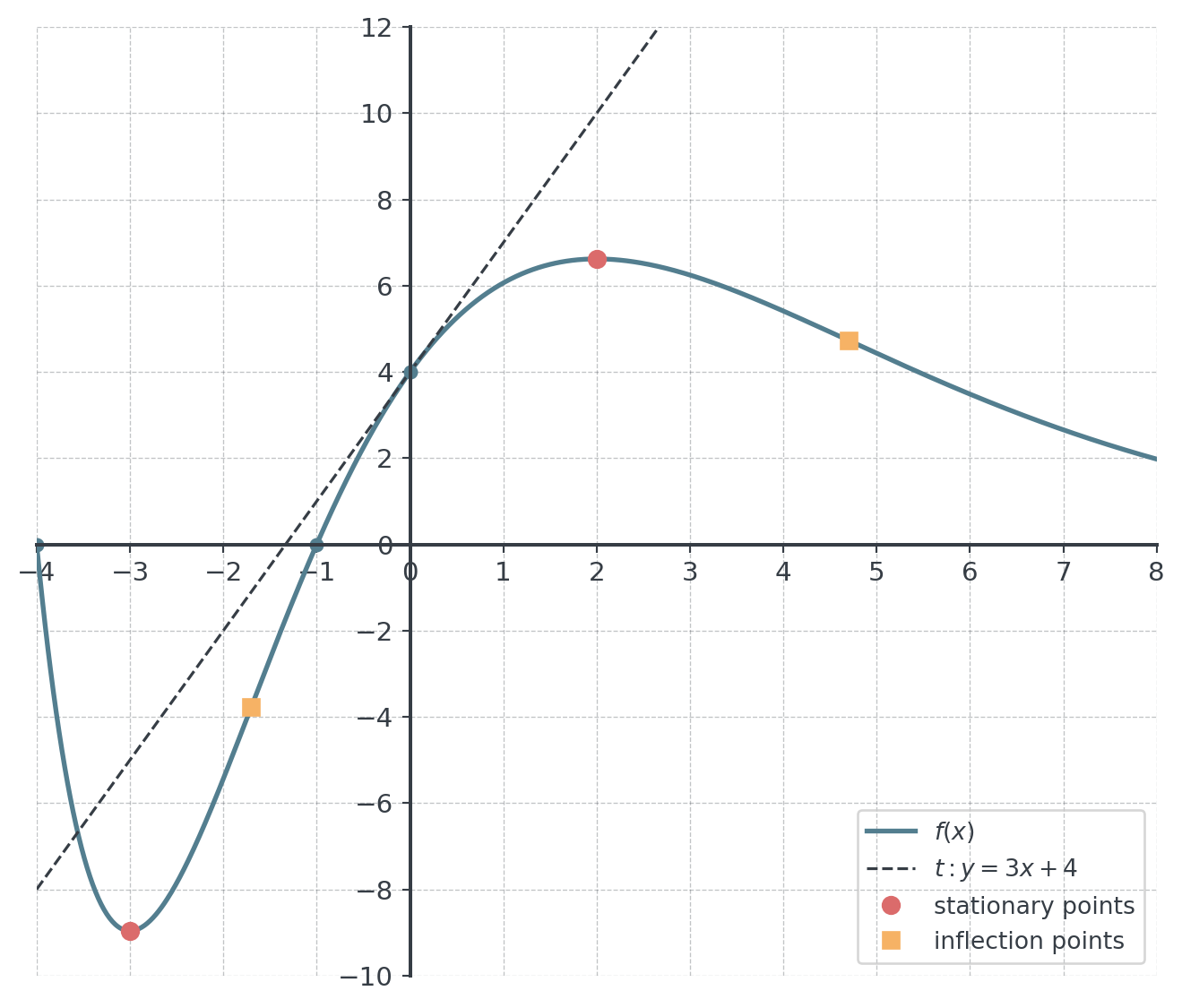
7. Determine the equation of the tangent \(t\) to the graph of \(f\) at its \(y\)-intercept. A line with slope \(m\) meets the \(x\)-axis at the angle \(\alpha = \arctan(m)\). Compute the angle of intersection \(\alpha\) between \(t\) and the \(x\)-axis.

Hint: The indicator D must show. SHIFT + tan gives \(\arctan\), just as SHIFT + sin gives \(\sin^{-1}\).

[5 pts.]

8. Argue whether the following statements are true or false.

(1) \(f\) has a global maximum at \(x = 2\).

(2) On the interval \([-1; 10]\), \(f\) takes its smallest value at \(x = -1\).

(3) The graph of \(f\) is concave down for every \(x > 2\).

(4) The graph of \(f\) is steeper at \(x = -1\) than at \(x = 0\).

[4 pts.]

1. Sketch the graph of \(f\) in the interval \([-4; 8]\) together with the tangent \(t\) from g). Mark the intercepts, the stationary points and the inflection points. [5 pts.]

CautionSolutions

a) Domain: \(x^2 + 5x + 4\) and \(e^{-0.5x}\) are defined for every real number, so \(D_f = \mathbb{R}\).

\(y\)-intercept: \(f(0) = 4 \cdot e^0 = 4\), i.e. \((0, 4)\).

\(x\)-intercepts: \(e^{-0.5x} > 0\) for every \(x\), so only the bracket can become zero:

\[x^2 + 5x + 4 = (x + 1)(x + 4) = 0 \iff x = -1 \text{ or } x = -4\]

The graph meets the \(x\)-axis at \((-4, 0)\) and \((-1, 0)\).

Grading: 1 Pt. domain, 1 Pt. \(y\)-intercept, 1 Pt. both \(x\)-intercepts with the reason \(e^{-0.5x} > 0\).

b) \(x \to \infty\): write \(f(x) = x^2 e^{-0.5x} + 5x e^{-0.5x} + 4e^{-0.5x}\). The exponential beats every power, \(x^n \cdot e^{-0.5x} \to 0\), so every term tends to 0:

\[\lim_{x \to \infty} f(x) = 0\]

\(x \to -\infty\): \(x^2 + 5x + 4 \to +\infty\) (the leading term \(x^2\) decides), and the exponent \(-0.5x\) tends to \(+\infty\), so \(e^{-0.5x} \to +\infty\):

\[\lim_{x \to -\infty} f(x) = +\infty\]

Horizontal asymptote: \(y = 0\) (the \(x\)-axis), only for \(x \to \infty\).

Far to the right: for \(x > -1\), both factors are positive, so \(f(x) > 0\). The graph approaches the \(x\)-axis from above, but it never reaches it.

Grading: 2 Pts. limit for \(x \to \infty\) with the reason, 1 Pt. limit for \(x \to -\infty\), 1 Pt. asymptote \(y = 0\) only on the right, 1 Pt. description (from above, never reached).

c) First derivative (product rule, and the chain rule for \(e^{-0.5x}\)): \(u = x^2 + 5x + 4\), \(v = e^{-0.5x}\), \(u' = 2x + 5\), \(v' = -0.5e^{-0.5x}\).

\[f'(x) = (2x + 5)e^{-0.5x} - 0.5(x^2 + 5x + 4)e^{-0.5x} = e^{-0.5x}(-0.5x^2 - 0.5x + 3)\]

Factor: \(-0.5x^2 - 0.5x + 3 = -0.5(x^2 + x - 6) = -0.5(x + 3)(x - 2)\), so

\[f'(x) = -0.5(x + 3)(x - 2) \cdot e^{-0.5x}\]

Second derivative (product rule on \(f'(x) = (-0.5x^2 - 0.5x + 3) \cdot e^{-0.5x}\), with \(u' = -x - 0.5\)):

\[f''(x) = (-x - 0.5)e^{-0.5x} - 0.5(-0.5x^2 - 0.5x + 3)e^{-0.5x} = e^{-0.5x}(0.25x^2 - 0.75x - 2)\]

\[f''(x) = 0.25(x^2 - 3x - 8) \cdot e^{-0.5x}\]

Grading: 1 Pt. \(u\), \(v\), \(u'\), \(v'\) with the chain rule, 1 Pt. \(f'(x)\) with the product rule, 1 Pt. factored form of \(f'\), 1 Pt. product rule for \(f''\), 1 Pt. simplified bracket, 1 Pt. \(f''(x)\).

d) Necessary condition: \(f'(x) = 0\). Since \(-0.5e^{-0.5x} \neq 0\):

\[(x + 3)(x - 2) = 0 \iff x = -3 \text{ or } x = 2\]

Second derivative test:

• \(f''(-3) = 0.25(9 + 9 - 8)e^{1.5} = 2.5e^{1.5} \approx 11.20 > 0\): local minimum
• \(f''(2) = 0.25(4 - 6 - 8)e^{-1} = -2.5e^{-1} \approx -0.92 < 0\): local maximum

Coordinates:

• \(f(-3) = (9 - 15 + 4)e^{1.5} = -2e^{1.5} \approx -8.96\): local minimum at \((-3, -8.96)\)
• \(f(2) = (4 + 10 + 4)e^{-1} = 18e^{-1} \approx 6.62\): local maximum at \((2, 6.62)\)

Grading: 1 Pt. necessary condition with \(e^{-0.5x} \neq 0\), 1 Pt. \(x = -3\) and \(x = 2\), 2 Pts. second derivative test at both points, 2 Pts. coordinates.

e) At least two.

• At the local minimum \(x = -3\) the graph is concave up, at the local maximum \(x = 2\) it is concave down. In between, the curvature changes sign: at least one inflection point lies between \(-3\) and \(2\).
• After the maximum, \(f\) falls and approaches the asymptote \(y = 0\) from above (b)). The graph has to level off, so \(f'\) must increase again towards 0, and the graph becomes concave up. The curvature changes sign a second time for some \(x > 2\).

Grading: 1 Pt. inflection point between the extrema with reason, 1 Pt. second inflection point from the asymptote with reason.

f) Necessary condition: \(f''(x) = 0\). Since \(0.25e^{-0.5x} \neq 0\):

\[x^2 - 3x - 8 = 0 \iff x = \frac{3 \pm \sqrt{9 + 32}}{2} = \frac{3 \pm \sqrt{41}}{2}, \qquad x_1 \approx -1.70, \quad x_2 \approx 4.70\]

Sign change: \(x^2 - 3x - 8\) is a parabola that opens upward. It is negative between its zeros and positive outside them, so \(f''\) changes its sign at \(x_1\) and at \(x_2\).

Coordinates: \(f(x_1) \approx -3.78\) and \(f(x_2) \approx 4.73\). The inflection points are \((-1.70, -3.78)\) and \((4.70, 4.73)\), one on each side of the maximum, as e) predicted.

Grading: 1 Pt. quadratic equation from \(f''(x) = 0\), 1 Pt. exact solutions, 1 Pt. sign change of \(f''\), 1 Pt. both coordinates.

g) Point of contact: the \(y\)-intercept \((0, 4)\) from a).

Slope: \(f'(0) = -0.5 \cdot 3 \cdot (-2) \cdot e^0 = 3\)

Tangent:

\[t: \; y = 3(x - 0) + 4 = 3x + 4\]

Angle of intersection:

\[\alpha = \arctan(3) \approx 71.57°\]

Grading: 1 Pt. point \((0, 4)\), 1 Pt. slope \(f'(0) = 3\), 1 Pt. equation of \(t\), 1 Pt. \(\alpha = \arctan(3)\), 1 Pt. \(71.57°\) (indicator D).

h)

1. False. \(f(x) \to +\infty\) for \(x \to -\infty\) (b)), e.g. \(f(-5) = 4e^{2.5} \approx 48.73 > 6.62\). The maximum at \(x = 2\) is only a local maximum.
2. True. \(f(-1) = 0\), and for \(-1 < x \leq 10\) the factors \(x + 1\), \(x + 4\) and \(e^{-0.5x}\) are all positive, so \(f(x) > 0\). (With the candidates: the only stationary point in the interval is the maximum at \(x = 2\), and the ends give \(f(-1) = 0\) and \(f(10) \approx 1.04\).)
3. False. By f), \(f''(x) > 0\) for \(x > 4.70\), e.g. \(f''(6) = 0.25 \cdot 10 \cdot e^{-3} > 0\). The graph is concave up there.
4. True. \(f'(-1) = -0.5 \cdot 2 \cdot (-3) \cdot e^{0.5} = 3e^{0.5} \approx 4.95\), and \(f'(0) = 3\). The slope at \(x = -1\) is larger.

Grading: 1 Pt. per statement (decision and reason).

i) Table of values (rounded to two decimal places):

\(x\)	\(-4\)	\(-3\)	\(-2\)	\(-1\)	\(0\)	\(1\)	\(2\)	\(3\)	\(4\)	\(6\)	\(8\)
\(f(x)\)	\(0\)	\(-8.96\)	\(-5.44\)	\(0\)	\(4\)	\(6.07\)	\(6.62\)	\(6.25\)	\(5.41\)	\(3.49\)	\(1.98\)

Figure 1: Graph of f with the tangent t at the y-intercept

Essential features: zeros at \(x = -4\) and \(x = -1\), \(y\)-intercept \((0, 4)\) with the tangent \(y = 3x + 4\), local minimum \((-3, -8.96)\), local maximum \((2, 6.62)\), inflection points \((-1.70, -3.78)\) and \((4.70, 4.73)\), and on the right the approach to the \(x\)-axis from above.

Grading: 1 Pt. labeled axes and a suitable scale on \([-4; 8]\), 1 Pt. intercepts and the tangent, 1 Pt. extrema, 1 Pt. inflection points with the correct curvature, 1 Pt. approach to \(y = 0\) on the right.

Problem 3: A Sales Season and a Function Family [25 pts. total]

Part A: Easter Bunnies

A confectionery sells chocolate Easter bunnies in the 10 weeks before Easter. It models the weekly sales \(t\) weeks after the start of the season by a polynomial of third degree \(S(t) = at^3 + bt^2 + ct + d\), with \(S\) in hundred bunnies per week. Last year’s season gives the following information:

• At the start of the season (\(t = 0\)), the confectionery sells 2,000 bunnies per week.
• The weekly sales grow fastest two weeks after the start of the season.
• Six weeks after the start, the weekly sales reach their highest value of 12,800 bunnies per week.

1. Write down the four equations for \(a\), \(b\), \(c\) and \(d\) that this information gives. Explain why the sentence about week 2 gives only one equation. [3 pts.]

2. Solve the system of equations and give \(S(t)\). [7 pts.]

(for verification: \(S(t) = -0.5t^3 + 3t^2 + 18t + 20\))

3. Show that \(S(t) = -0.5(t - 10)(t + 2)^2\), and explain what the zero \(t = 10\) means for the season. Compute by how much the weekly sales grow per week at the moment of the fastest growth. [3 pts.]

Part B: A Function Family

For every \(k > 0\), the function \(g_k\) is given by

\[g_k(x) = e^x - kx, \quad x \in \mathbb{R}\]

4. Show that every function \(g_k\) has exactly one stationary point, at \(x = \ln(k)\). [2 pts.]

5. Prove that this stationary point is a local minimum for every \(k > 0\), and show that its \(y\)-value is \(k(1 - \ln(k))\). Show that all graphs of the family pass through the same point. [3 pts.]

6. Determine \(k\) so that the minimum lies at \(x = 2\), and give the coordinates of this minimum. [2 pts.]

7. Determine \(k\) so that the minimum lies on the \(x\)-axis, and give this lowest point. [2 pts.]

8. Explain why \(g_k\) has no zero for \(0 < k < e\), and why \(g_e\) has exactly one zero. [3 pts.]

CautionSolutions

a) With \(S'(t) = 3at^2 + 2bt + c\) and \(S''(t) = 6at + 2b\):

1. Start of the season: 2,000 bunnies \(= 20\) hundred, so \(S(0) = 20\), i.e. \(d = 20\)
2. Fastest growth at \(t = 2\): the growth rate \(S'\) is highest there, so \(S''(2) = 0\), i.e. \(12a + 2b = 0\)
3. Highest weekly sales at \(t = 6\): \(S'(6) = 0\), i.e. \(108a + 12b + c = 0\)
4. Their value, 12,800 bunnies \(= 128\) hundred: \(S(6) = 128\), i.e. \(216a + 36b + 6c + d = 128\)

The sentence about week 2 only says where the weekly sales grow fastest: the growth rate \(S'\) has its maximum there, so \(S\) has an inflection point at \(t = 2\). It gives neither the sales \(S(2)\) nor the growth rate \(S'(2)\), so it gives only one equation, \(S''(2) = 0\).

Grading: 1 Pt. \(d = 20\) and \(S''(2) = 0\), 1 Pt. \(S'(6) = 0\) and \(S(6) = 128\), 1 Pt. explanation (only the location of the inflection point is known, no value).

b) Solving (with \(d = 20\) a 3×3 system):

• From 2: \(b = -6a\)
• Into 3: \(108a - 72a + c = 0\), so \(c = -36a\)
• Into 4: \(216a + 36(-6a) + 6(-36a) + 20 = 128\), so \(216a - 216a - 216a = 108\), i.e. \(-216a = 108\) and \(a = -0.5\)
• Back-substitute: \(b = 3\), \(c = 18\)

\[S(t) = -0.5t^3 + 3t^2 + 18t + 20\]

Check: \(S''(t) = -3t + 6\), so \(S''(2) = 0\) ✓. \(S'(t) = -1.5t^2 + 6t + 18\), so \(S'(6) = -54 + 36 + 18 = 0\) ✓. \(S(6) = -108 + 108 + 108 + 20 = 128\) ✓.

Grading: 1 Pt. \(b = -6a\), 1 Pt. \(c = -36a\), 2 Pts. equation for \(a\) and \(a = -0.5\), 1 Pt. \(b\) and \(c\), 1 Pt. \(S(t)\), 1 Pt. check.

c) Expand:

\[-0.5(t - 10)(t + 2)^2 = -0.5(t - 10)(t^2 + 4t + 4) = -0.5(t^3 - 6t^2 - 36t - 40) = -0.5t^3 + 3t^2 + 18t + 20 \quad \checkmark\]

Meaning of \(t = 10\): \(S(10) = 0\), and \(S(t) > 0\) for \(0 \leq t < 10\) (only the factor \(t - 10\) is negative there). Ten weeks after the start, at Easter, the weekly sales have fallen to zero: the season ends.

Fastest growth: \(S'(2) = -6 + 12 + 18 = 24\) hundred bunnies per week, per week. At the moment of the fastest growth, the weekly sales grow by about 2,400 bunnies per week.

Grading: 1 Pt. expansion, 1 Pt. meaning of \(t = 10\), 1 Pt. \(S'(2) = 24\) with the unit.

d) Derivative: \(g_k'(x) = e^x - k\).

Stationary points: \(g_k'(x) = 0 \iff e^x = k \iff x = \ln(k)\). Since \(k > 0\), \(\ln(k)\) exists, and it is the only solution: every \(g_k\) has exactly one stationary point.

Grading: 1 Pt. \(g_k'(x)\), 1 Pt. \(x = \ln(k)\) as the only solution.

e) Nature: \(g_k''(x) = e^x > 0\) for every \(x\), so \(g_k''(\ln(k)) = k > 0\): a local minimum, for every \(k > 0\).

\(y\)-value: with \(e^{\ln(k)} = k\):

\[g_k(\ln(k)) = e^{\ln(k)} - k\ln(k) = k - k\ln(k) = k(1 - \ln(k)) \quad \checkmark\]

Common point: \(g_k(0) = e^0 - k \cdot 0 = 1\) for every \(k > 0\). All graphs of the family pass through the point \((0, 1)\).

Grading: 1 Pt. \(g_k'' > 0\) and minimum, 1 Pt. \(y\)-value with \(e^{\ln(k)} = k\), 1 Pt. \(g_k(0) = 1\) for every \(k\), common point \((0, 1)\).

f) \(\ln(k) = 2 \iff k = e^2 \approx 7.39\). The minimum is \(\left(2, e^2(1 - 2)\right) = (2, -e^2) \approx (2, -7.39)\).

Grading: 1 Pt. \(k = e^2\), 1 Pt. coordinates.

g) The \(y\)-value must be 0: \(k(1 - \ln(k)) = 0\). Since \(k > 0\), \(1 - \ln(k) = 0 \iff \ln(k) = 1 \iff k = e\). The lowest point is \((\ln(e), 0) = (1, 0)\).

Grading: 1 Pt. \(k = e\), 1 Pt. lowest point \((1, 0)\).

h) \(g_k'(x) = e^x - k\) is negative for \(x < \ln(k)\) and positive for \(x > \ln(k)\), because \(e^x\) grows. So \(g_k\) falls up to the minimum and rises after it: the minimum is the lowest point of the whole graph.

• \(0 < k < e\): then \(\ln(k) < 1\), so \(1 - \ln(k) > 0\) and the lowest value \(k(1 - \ln(k))\) is positive. All values of \(g_k\) are positive: no zero.
• \(k = e\): the lowest value is 0, at \(x = 1\) (g)). Every other value is larger than 0, so \(x = 1\) is the only zero: the graph touches the \(x\)-axis there.

Grading: 1 Pt. minimum is the lowest point (sign of \(g_k'\)), 1 Pt. no zero for \(0 < k < e\), 1 Pt. exactly one zero for \(k = e\).

Exam Preparation Checklist

Before the exam, ensure you can:

• Compute limits from a graph, by factoring and cancelling and for \(x \to \pm\infty\), and check continuity with the three conditions
• Tell a hole (removable discontinuity) from a vertical asymptote with one-sided limits
• Compute the slope of a secant and the tangential gradient, and interpret marginal cost, marginal revenue and marginal profit
• Differentiate with the power, product, quotient and chain rules, including \(e^x\), \(e^{g(x)}\) and \(\ln(x)\), and check a derivative value with the d/dx template
• Investigate the asymptotic behavior of functions like \((x^2 + bx + c) \cdot e^{-kx}\) with \(x^n \cdot e^{-kx} \to 0\) for \(x \to \infty\)
• Determine the nature and the coordinates of all stationary points with the sign change of \(f'\) or the second derivative test, and recognize a saddle point
• Determine inflection points with \(f''\) (sign change or \(f'''\)), assess how many inflection points a function has to possess at least, and explain their meaning, e.g. the fastest growth or the lowest marginal costs
• Determine a tangent or an inflectional tangent and the angle of intersection \(\alpha = \arctan(m)\) with the indicator D
• Find global extrema on a closed interval with the values at the ends, e.g. the highest profit within the capacity
• Sketch a graph with the 6-step algorithm and argue whether statements about \(f\), \(f'\) and \(f''\) are true or false
• Determine a cubic cost, revenue or sales function from conditions: an extremum or a tangent gives two equations, an inflectional tangent three
• Get the cost function from the marginal costs and the fixed costs
• Compute the maximum profit, prove that it is a maximum and give the price, and determine the break-even point and the profit limit
• Compute the lowest unit costs, the long-term price floor and the short-term lower limit price, and decide with them
• Work with a function family: stationary points in terms of the parameter, and the parameter for a given location or value

Remember: Show all work, label units, and interpret your results in the business context.