Consulting Project: TechMart Inventory Optimization

Management Science - E-commerce Inventory Management

Client Briefing: TechMart Electronics

Meet Your Client

  • Industry: E-commerce / Electronics Retail
  • Client Contact: Yola Wang, Chief Operations Officer
  • Company Size: 200 employees
  • Market: Consumer electronics in Germany

The COO’s Inventory Crisis

Yola Wang, COO of TechMart

“We’re drowning in inventory but constantly out of stock on bestsellers. It makes no sense!

Here’s our situation: We sell 30 electronics SKUs online: smartphones, laptops, headphones, smartwatches, tablets. We have two warehouses:

  • Fast Warehouse (Hamburg): Right next to our shipping hub. Orders ship in 1-2 hours. But it’s small and has only 8,000 unit capacity.
  • Large Warehouse (Poland): Huge storage (50,000+ capacity) but orders take 2-3 days to ship from there.

The problem? We’re making terrible allocation decisions:

  • Slow-movers occupy 40% of fast warehouse space
  • Shipping delays costing us hundreds of thousands annually in customer refunds
  • Customer complaints about “2-day delivery” are up 60%

Black Friday is in 3 weeks. Last year was a disaster… We ran out of top items in the fast warehouse on Day 1, then spent a week scrambling with slow shipping from Poland. Lost a lot of potential revenue.

Here’s the critical constraint: Once Black Friday starts, we CANNOT refill the Hamburg warehouse. All our warehouse staff are 100% busy picking and packing orders and there’s zero time for restocking. Whatever allocation we make beforehand is what we’re stuck with for the entire weeks!

I need you to:

  1. Forecast Black Friday demand for each SKU (weeks 47-48)
  2. Decide which SKUs (and how many units) to pre-position in the fast warehouse (limited to 8,000 units!)
  3. Minimize shipping delay costs
  4. Show me the business impact in €€€

I have 3 years of sales history. Can you help us get this right before Black Friday?“

The Business Context

Warehouse System

Fast Warehouse (Hamburg)

  • Capacity: 8,000 units total
  • Shipping speed: 1-2 hours processing, next-day delivery
  • Storage cost: €2.50 per unit (for Black Friday period)
  • Perfect for: High-demand, fast-moving items

Large Warehouse (Poland)

  • Capacity: 50,000+ units (effectively unlimited for our needs)
  • Shipping speed: 2-3 days processing, 2-3 days delivery (4-6 days total!)
  • Storage cost: €0.80 per unit (for Black Friday period)
  • Perfect for: Slow-movers, bulk storage

The Allocation Problem

Before Black Friday:

You must decide how many units of each SKU to pre-position in the fast warehouse (Hamburg) vs. large warehouse (Poland).

Critical Constraints:

  • Total units in fast warehouse ≤ 8,000
  • No refilling during Black Friday! All warehouse staff are busy handling the surge, whatever you allocate is fixed for the entire weekend

During Black Friday:

  • Units in Fast Warehouse (Hamburg): Ship quickly (1-2 days), customers happy, no delay penalty
  • Units in Large Warehouse (Poland): Ship slowly (4-6 days), customers complain, delay penalty applies

Your Goal: Decide how many units of each SKU go in Hamburg warehouse to minimize total delay penalty costs. Note: While storage costs differ, Yola cares most about customer satisfaction. Minimize the delay penalties first.

Note, we have sufficient total inventory of each SKU. The question is WHERE to store each unit before Black Friday!

Example Allocation:

SKU-001: 450 units in Hamburg, rest in Poland
SKU-002: 380 units in Hamburg, rest in Poland
SKU-003: 0 units in Hamburg, all in Poland
...
SKU-030: 200 units in Hamburg, rest in Poland
Total: ≤ 8,000 units in Hamburg

Cost Structure

Delay Penalty (per unit from Poland warehouse):

  • 15% of customers cancel order: lost sale (50 % of product price as opportunity costs)
  • 85% of customers wait but demand partial refund: €10 compensation

Customer Expectations

  • High-demand items: Customers expect 1-2 day delivery (Hamburg warehouse)
  • Low-demand items: Customers more tolerant of 4-6 day delivery (Poland warehouse)
  • Black Friday: Everyone expects fast delivery! High delay costs for all SKUs.

The Data: 3 Years of Sales History

import numpy as np
import pandas as pd
import matplotlib.pyplot as plt
from datetime import datetime, timedelta

# Set random seed for reproducibility
np.random.seed(2025)

def generate_techmart_sales_history():
    """
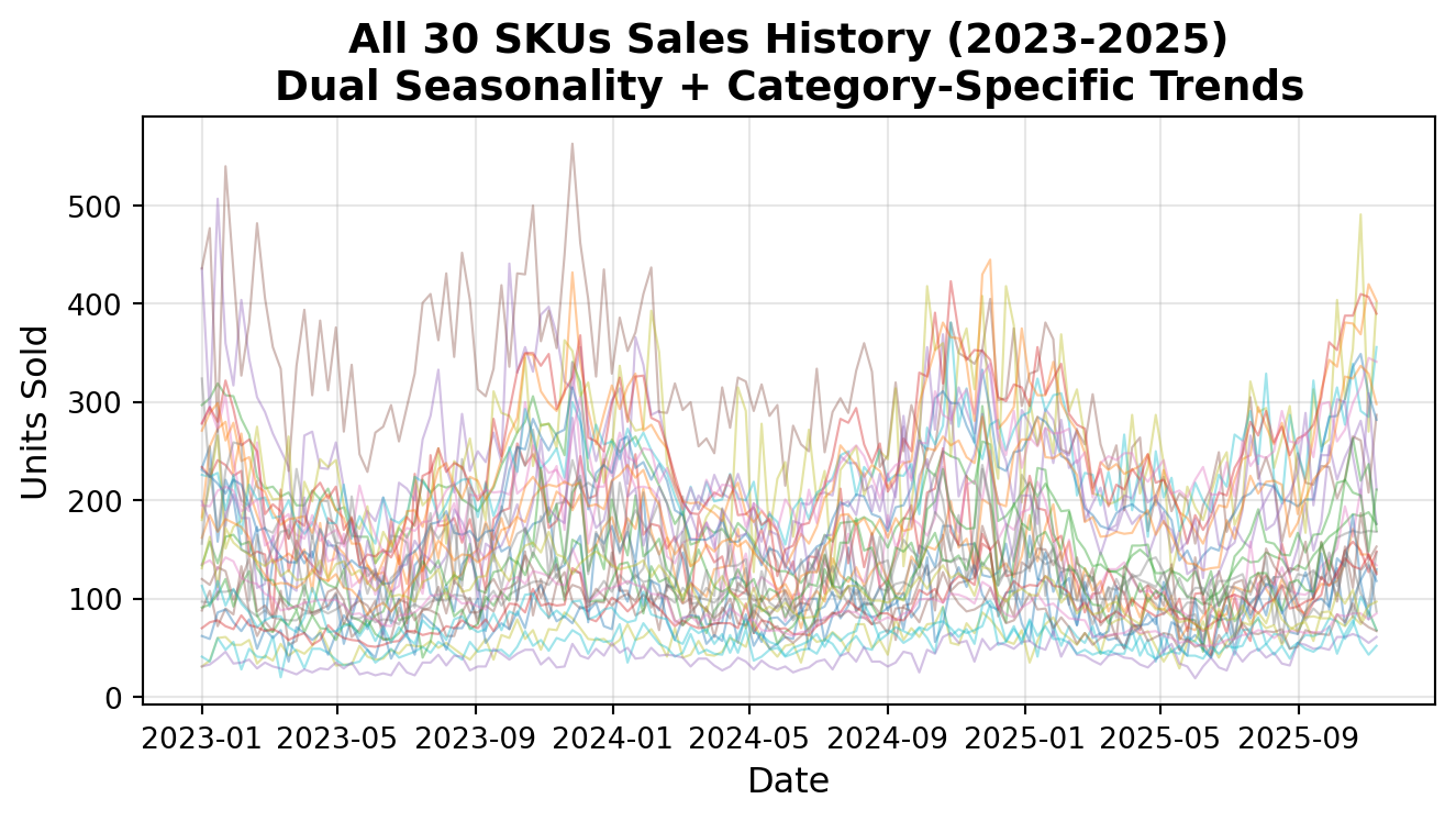
    Generate 3 years of sales history for 30 electronics SKUs.
    """

    # Define 30 SKUs across 5 categories with category-specific trends
    # Trend: annual growth/decline rate (e.g., 0.05 = 5% growth per year)
    categories = {
        'Smartphones': {'count': 8, 'trend': -0.15},  # Mature market, slight decline
        'Laptops': {'count': 6, 'trend': 0.11},       # Stable with slight growth
        'Headphones': {'count': 6, 'trend': 0.18},    # Growing premium audio market
        'Smartwatches': {'count': 5, 'trend': 0.22},  # Emerging category, strong growth
        'Tablets': {'count': 5, 'trend': -0.15}       # Declining market
    }

    skus = []
    sku_id = 1
    for category, cat_info in categories.items():
        count = cat_info['count']
        category_trend = cat_info['trend']

        for i in range(count):
            # Each product has unique characteristics
            if category == 'Smartphones':
                base_demand = np.random.uniform(100, 410)
            elif category == 'Laptops':
                base_demand = np.random.uniform(90, 220)
            elif category == 'Headphones':
                base_demand = np.random.uniform(20, 210)
            elif category == 'Smartwatches':
                base_demand = np.random.uniform(20, 140)
            elif category == 'Tablets':
                base_demand = np.random.uniform(80, 170)

            # Seasonal strength: how much seasonality affects this product (0.1-0.3)
            seasonal_strength = np.random.uniform(0.1, 0.3)

            # Noise level: product-specific volatility (std: 0.08-0.20)
            noise_std = np.random.uniform(0.03, 0.25)

            # Black Friday boost: product-specific multiplier (1.1-1.5)
            bf_multiplier = np.random.uniform(1.1, 1.5)

            skus.append({
                'sku_id': f'SKU-{sku_id:03d}',
                'category': category,
                'base_demand': base_demand,
                'seasonal_strength': seasonal_strength,
                'noise_std': noise_std,
                'bf_multiplier': bf_multiplier,
                'category_trend': category_trend,
                'price': np.random.uniform(30, 1200)
            })
            sku_id += 1

    skus_df = pd.DataFrame(skus)

    # Generate weekly sales from 2023-01-01 to 2025-11-15 (almost 3 years)
    start_date = datetime(2023, 1, 1)
    end_date = datetime(2025, 11, 15)
    weeks = pd.date_range(start_date, end_date, freq='W')

    sales_data = []

    for _, sku in skus_df.iterrows():
        for week_start in weeks:
            week_num = week_start.isocalendar()[1]
            year = week_start.year
            month = week_start.month

            # Base demand (unique per product)
            demand = sku['base_demand']

            # Component 1: Category-specific trend (small, linear over time)
            # Calculate years elapsed from start date (2023-01-01)
            years_elapsed = (week_start - start_date).days / 365.25
            trend_multiplier = 1.0 + (sku['category_trend'] * years_elapsed)
            demand *= trend_multiplier

            # Component 2: Annual cycle (52 weeks) - peak in Nov/Dec (Q4), trough in summer (Q3)
            annual_seasonality = 1.0 + sku['seasonal_strength'] * np.cos(2 * np.pi * (week_num - 47) / 52)

            # Component 3: Quarterly cycle (13 weeks) - shorter-term fluctuations
            quarterly_seasonality = 1.0 + (sku['seasonal_strength'] * 0.5) * np.sin(2 * np.pi * week_num / 13)

            demand *= annual_seasonality * quarterly_seasonality

            # Black Friday boost (product-specific multiplier)
            if week_num in [47, 48]:
                demand *= sku['bf_multiplier']

            # Add normally distributed random noise (product-specific volatility)
            noise = np.random.normal(1.0, sku['noise_std'])
            demand *= max(0.5, min(1.5, noise))  # Clip to reasonable range

            # Round to integer
            demand = max(0, int(demand))

            sales_data.append({
                'sku_id': sku['sku_id'],
                'week_start': week_start,
                'year': year,
                'week': week_num,
                'month': month,
                'units_sold': demand
            })

    sales_df = pd.DataFrame(sales_data)

    return skus_df, sales_df

# Generate data
skus_df, sales_df = generate_techmart_sales_history()

print("TECHMART ELECTRONICS - SKU CATALOG")
print("=" * 120)
print(skus_df.to_string(index=False))
print("\n" + "=" * 120)
print(f"Total SKUs: {len(skus_df)}")
print("\nBy category:")
for category in skus_df['category'].unique():
    count = len(skus_df[skus_df['category'] == category])
    print(f"  {category}: {count} SKUs")
TECHMART ELECTRONICS - SKU CATALOG
========================================================================================================================
 sku_id     category  base_demand  seasonal_strength  noise_std  bf_multiplier  category_trend       price
SKU-001  Smartphones   142.001331           0.277570   0.235173       1.278227           -0.15  484.235589
SKU-002  Smartphones   179.854895           0.231474   0.138376       1.485695           -0.15  967.151836
SKU-003  Smartphones   241.113638           0.260212   0.039178       1.407783           -0.15   33.710207
SKU-004  Smartphones   190.770912           0.222183   0.230866       1.220046           -0.15  320.860405
SKU-005  Smartphones   306.581553           0.297507   0.133019       1.149315           -0.15 1101.756722
SKU-006  Smartphones   393.304495           0.155539   0.144324       1.161898           -0.15   47.114003
SKU-007  Smartphones   200.515394           0.298180   0.142891       1.450598           -0.15  108.853024
SKU-008  Smartphones   188.087659           0.193780   0.197590       1.469045           -0.15  489.837796
SKU-009      Laptops   210.781398           0.199922   0.206451       1.458632            0.11  594.091018
SKU-010      Laptops   200.230887           0.155336   0.104850       1.142030            0.11  642.082831
SKU-011      Laptops   174.306043           0.279922   0.052851       1.224698            0.11  121.380883
SKU-012      Laptops   211.923125           0.291817   0.072073       1.481608            0.11  549.536481
SKU-013      Laptops   124.245171           0.233980   0.112779       1.494186            0.11  810.475763
SKU-014      Laptops   218.890762           0.294713   0.069920       1.276549            0.11  817.168259
SKU-015   Headphones   144.177841           0.176608   0.177231       1.387934            0.18  946.536415
SKU-016   Headphones    80.986683           0.119412   0.213572       1.110089            0.18  309.358839
SKU-017   Headphones   182.850584           0.110092   0.072704       1.290362            0.18  305.164876
SKU-018   Headphones    88.229309           0.129033   0.059840       1.139115            0.18  207.471104
SKU-019   Headphones    47.458748           0.105895   0.190427       1.370478            0.18  548.940060
SKU-020   Headphones    43.726319           0.135155   0.164134       1.208759            0.18  863.933878
SKU-021 Smartwatches    63.921751           0.155961   0.223931       1.166687            0.22  147.990342
SKU-022 Smartwatches   136.894623           0.291290   0.057567       1.152603            0.22  428.359589
SKU-023 Smartwatches    80.065334           0.269516   0.155000       1.186574            0.22  757.086860
SKU-024 Smartwatches    66.345697           0.176956   0.071607       1.482957            0.22  174.054069
SKU-025 Smartwatches    30.384036           0.220347   0.161101       1.150430            0.22  749.579075
SKU-026      Tablets   109.464296           0.169059   0.104956       1.148955           -0.15 1140.611174
SKU-027      Tablets   111.850145           0.198087   0.043744       1.295709           -0.15  439.401212
SKU-028      Tablets   166.496499           0.152798   0.191875       1.299498           -0.15 1114.312833
SKU-029      Tablets   140.870051           0.114547   0.087424       1.174714           -0.15  783.925103
SKU-030      Tablets    85.573274           0.168057   0.138067       1.413962           -0.15   71.210130

========================================================================================================================
Total SKUs: 30

By category:
  Smartphones: 8 SKUs
  Laptops: 6 SKUs
  Headphones: 6 SKUs
  Smartwatches: 5 SKUs
  Tablets: 5 SKUs

Sales History Overview

print("\nSALES HISTORY SUMMARY")
print("=" * 80)
print(f"Date range: {sales_df['week_start'].min().date()} to {sales_df['week_start'].max().date()}")
print(f"Total weeks: {sales_df['week_start'].nunique()}")
print(f"Total records: {len(sales_df):,}")
print(f"Total units sold (3 years): {sales_df['units_sold'].sum():,}")

# Show sample of sales data
print("\nSample sales data (first 20 records):")
print(sales_df.head(20).to_string(index=False))

SALES HISTORY SUMMARY
================================================================================
Date range: 2023-01-01 to 2025-11-09
Total weeks: 150
Total records: 4,500
Total units sold (3 years): 674,482

Sample sales data (first 20 records):
 sku_id week_start  year  week  month  units_sold
SKU-001 2023-01-01  2023    52      1         233
SKU-001 2023-01-08  2023     1      1         255
SKU-001 2023-01-15  2023     2      1         158
SKU-001 2023-01-22  2023     3      1         221
SKU-001 2023-01-29  2023     4      1         202
SKU-001 2023-02-05  2023     5      2         150
SKU-001 2023-02-12  2023     6      2         146
SKU-001 2023-02-19  2023     7      2         173
SKU-001 2023-02-26  2023     8      2          78
SKU-001 2023-03-05  2023     9      3         138
SKU-001 2023-03-12  2023    10      3         143
SKU-001 2023-03-19  2023    11      3          93
SKU-001 2023-03-26  2023    12      3         150
SKU-001 2023-04-02  2023    13      4         136
SKU-001 2023-04-09  2023    14      4         148
SKU-001 2023-04-16  2023    15      4         117
SKU-001 2023-04-23  2023    16      4          89
SKU-001 2023-04-30  2023    17      4         104
SKU-001 2023-05-07  2023    18      5          54
SKU-001 2023-05-14  2023    19      5          81

Warehouse Capacity Analysis

# Analyze capacity feasibility
warehouses = {
    'Fast Warehouse (Hamburg)': {
        'capacity': 8000,  # units
        'description': 'Premium location, fast shipping, limited space'
    },
    'Large Warehouse (Poland)': {
        'capacity': 100000,  # 50000 units (effectively unlimited)
        'description': 'Cheap storage, slow shipping, huge space'
    }
}

print("\nWAREHOUSE SPECIFICATIONS")
print("=" * 80)
for warehouse, specs in warehouses.items():
    print(f"\n{warehouse}:")
    for key, value in specs.items():
        if key != 'description':
            print(f"  {key}: {value}")
    print(f"  → {specs['description']}")

print("\n" + "=" * 80)
print("KEY CONSTRAINT: Fast warehouse can only hold 8,000 units total!")
print("\nALLOCATION DECISION:")
print("  - You must forecast Black Friday demand for each SKU")
print("  - Then decide which SKUs to store in fast warehouse")
print("  - Goal: Minimize total delay costs!")

WAREHOUSE SPECIFICATIONS
================================================================================

Fast Warehouse (Hamburg):
  capacity: 8000
  → Premium location, fast shipping, limited space

Large Warehouse (Poland):
  capacity: 100000
  → Cheap storage, slow shipping, huge space

================================================================================
KEY CONSTRAINT: Fast warehouse can only hold 8,000 units total!

ALLOCATION DECISION:
  - You must forecast Black Friday demand for each SKU
  - Then decide which SKUs to store in fast warehouse
  - Goal: Minimize total delay costs!

Minimal Helper Functions

We provide only basic data access and cost calculation functions. You must implement forecasting, optimization, and simulation yourself.

def get_sku_sales_history(sku_id, sales_df):
    """
    Get sales history for a specific SKU.

    Args:
        sku_id: SKU identifier (e.g., 'SKU-001')
        sales_df: DataFrame with sales history

    Returns:
        DataFrame with weekly sales for the SKU
    """
    return sales_df[sales_df['sku_id'] == sku_id].sort_values('week_start').reset_index(drop=True)
def plot_sku_sales_trend(sku_id, sales_df, skus_df):
    """Plot sales trend for a specific SKU."""
    sku_history = get_sku_sales_history(sku_id, sales_df)
    sku_info = skus_df[skus_df['sku_id'] == sku_id].iloc[0]

    plt.figure(figsize=(14, 5))
    plt.plot(sku_history['week_start'], sku_history['units_sold'], linewidth=1.5)
    plt.axhline(y=sku_info['base_demand'], color='red', linestyle='--',
                label=f'Base Demand: {sku_info["base_demand"]}', alpha=0.7)

    # Highlight Black Friday weeks
    bf_weeks = sku_history[sku_history['week'].isin([47, 48])]
    plt.scatter(bf_weeks['week_start'], bf_weeks['units_sold'],
                color='orange', s=100, zorder=5, label='Black Friday')

    plt.xlabel('Date', fontsize=12)
    plt.ylabel('Units Sold', fontsize=12)
    plt.title(f'{sku_id} Sales History - {sku_info["category"]} (Base: {sku_info["base_demand"]} units/week)',
              fontsize=14, fontweight='bold')
    plt.legend()
    plt.grid(True, alpha=0.3)
    plt.tight_layout()
    plt.show()

# Plot all SKUs together to visualize the dual seasonality pattern
plt.figure()

for sku_id in skus_df['sku_id']:
    sku_history = get_sku_sales_history(sku_id, sales_df)
    sku_info = skus_df[skus_df['sku_id'] == sku_id].iloc[0]
    plt.plot(sku_history['week_start'], sku_history['units_sold'],
            alpha=0.4, linewidth=0.8)

plt.xlabel('Date', fontsize=12)
plt.ylabel('Units Sold', fontsize=12)
plt.title('All 30 SKUs Sales History (2023-2025)\nDual Seasonality + Category-Specific Trends',
         fontsize=14, fontweight='bold')
plt.grid(True, alpha=0.3)
plt.tight_layout()
plt.show()

Your Task

You must develop an inventory optimization solution that forecasts Black Friday demand and optimally allocates SKUs to warehouses. Provide:

1. Jupyter Notebook with Complete Solution

Your notebook should include:

  • Exploratory Data Analysis:

    • Seasonality patterns (visualize aggregate sales over time)
    • Product lifecycle trends
    • Black Friday spike analysis (2023 vs 2024)
    • SKU categorization (fast-movers vs. slow-movers)
  • Demand Forecasting:

    • Forecast Black Friday 2025 demand (weeks 47-48 combined) for all 30 SKUs
    • Report forecast accuracy metrics (MAE, RMSE, or MAPE)
  • Inventory Allocation Optimization:

    • Decision: How many units of each SKU to allocate to Hamburg warehouse (total ≤ 8,000 units!)
    • Objective: Minimize total delay cost
  • Monte Carlo Simulation:

    • Generate 10,000 demand scenarios from your forecast with a variation defined by you
    • For each scenario, calculate total delay cost using your fixed allocation
    • Analyze: Mean cost, standard deviation, 95th percentile (worst-case)
    • Insight: How robust is your allocation to forecast errors?
  • Results & Business Impact:

    • Total expected delay cost
    • Allocation breakdown: How many units of each SKU in Hamburg vs. Poland
    • Comparison to baseline (e.g., equal allocation across all SKUs, or random)
    • Cost savings in €€€

I won’t judge the code quality in this notebook. It’s just for me to review your final solution and identify any mistakes if your results seem unrealistic. The final project will be graded primarily based on your presentation and the results you have achieved.

2. Presentation

  • Problem understanding: Yola’s crisis in your own words
  • Your approach: Forecasting method + allocation logic
  • Results: Forecasts, allocation decision, Monte Carlo analysis
  • Business impact: savings, recommendations, trade-offs, limitations

Please upload both, presentation and jupyter notebook (or .py files) for the final project.

3. Key Metrics to Report

  • Forecasting: Forecast accuracy and forecasted demand for 2025 Black Friday
  • Allocation: Total units allocated to fast warehouse (must be ≤ 8,000!)
  • Expected cost: Total delay Costs based on allocation decision
  • Monte Carlo Risk Analysis: Report all important metrics (your choice) and 95th percentile cost
  • Business Impact: Cost savings vs. baseline allocation

Constraints and Requirements

Hard Constraints (Must Satisfy)

  1. Capacity: Total forecasted demand allocated to fast warehouse ≤ 8,000 units

Soft Constraints (Optimize)

  1. Minimize delay costs: Fewer units in Poland = lower total cost
  2. Robustness: Allocation should perform reasonably under demand uncertainty (Monte Carlo)

Tips for Success

  1. No refilling during Black Friday! Your allocation is fixed for the entire weekend.
  2. Forecasting is critical: A 10% forecast error can shift which SKUs get priority.
  3. Monte Carlo reveals risk: Your allocation might have same expected cost but higher variance.
  4. Start simple, iterate: Get a working forecast → simple allocation → validate → Monte Carlo

Common Pitfalls to Avoid

  • Overfitting forecast: Don’t overfit to historical data. Use simple, robust methods.
  • Ignoring capacity: Double-check that total allocated to fast warehouse ≤ 8,000!
  • Poor visualization: Make your allocation decision clear (how many units of each SKU where?)
  • No baseline comparison: Always compare to a baseline (e.g., random allocation) to show improvement

Data Access

All data is provided in this notebook:

  • skus_df: DataFrame with 30 SKUs and their attributes
  • sales_df: DataFrame with 3 years of weekly sales history
  • warehouses: Dict with warehouse specifications
  • Helper functions: get_sku_sales_history(), plot_sku_sales_trend()

You must implement forecasting, allocation optimization, and Monte Carlo simulation yourself!

Deadline

  • Notebook submission & Presentation: Lecture 12
  • Good luck, consultants!