Welcome back to Bean Counter, CEO! In the lecture, we saw how Monte Carlo simulation helps us make decisions when the future is uncertain. Now it’s time to apply these techniques to expand your coffee empire and prepare for the TechVenture competition.
Your CEO Challenge: Bean Counter Expansion - analyzing single locations and portfolios for strategic growth
Key Skills for Competition:
Simulating uncertain returns
Analyzing risk metrics
Comparing portfolio combinations
Making data-driven recommendations
import numpy as npimport pandas as pdimport matplotlib.pyplot as pltfrom itertools import combinations # Allows us to generate all portfolio combinations# Set seed for reproducibilitynp.random.seed(42)print("Libraries loaded! Let's analyze Bean Counter expansion opportunities ☕")
Section 1 - Modeling Uncertainty with Distributions
Let’s start by modeling uncertain business variables using probability distributions.
Understanding np.random
# Example: Daily customer traffic follows a normal distribution# Historical data shows: mean = 100, std = 20# Simulate one dayone_day_customers = np.random.normal(100, 20)print(f"One random day: {one_day_customers:.0f} customers")# Simulate many days to see the patternmany_days = np.random.normal(100, 20, size=1000)print(f"\n1000 days simulation:")print(f" Mean: {many_days.mean():.1f} (expected: 100)")print(f" Std Dev: {many_days.std():.1f} (expected: 20)")print(f" Min: {many_days.min():.0f}, Max: {many_days.max():.0f}")
One random day: 110 customers

1000 days simulation:
  Mean: 100.4 (expected: 100)
  Std Dev: 19.6 (expected: 20)
  Min: 35, Max: 177
Exercise 1.1 - Simulate Purchase Amounts
Average purchase per customer varies uniformly between €8 and €12. Simulate 10,000 purchase amounts.
# YOUR CODE BELOW# Simulate 10,000 purchase amounts uniformly distributed between 8 and 12purchase_amounts =# Calculate statisticsmean_purchase =min_purchase =max_purchase =
Code
# Don't modify below - these test your solutionassertlen(purchase_amounts) ==10_000, "Should have 10,000 simulations"assert9.9< mean_purchase <10.1, f"Mean should be ~10, got {mean_purchase:.2f}"assert8<= min_purchase <9, f"Min should be ~8, got {min_purchase:.2f}"assert11< max_purchase <=12, f"Max should be ~12, got {max_purchase:.2f}"print("Great, the purchase simulation is correct!")
Exercise 1.2 - Calculate Probabilities
Using your simulated data from the previous task, calculate key probabilities.
NoteBoolean Operations and Probabilities
# Create boolean array (True/False)data = np.array([50, 150, 80, 200])high_values = data >100# [False, True, False, True]# Calculate probability: mean of boolean = proportion of Trueprob = (data >100).mean() # 0.5 = 50%# Combine conditions with & (and) or | (or)prob_range = ((data >=80) & (data <=150)).mean()
# YOUR CODE BELOW# Using the many_days array from above (1000 days of customer data)# Calculate the probability of different scenarios# Probability of getting more than 120 customersprob_high =# Probability of getting fewer than 80 customersprob_low =# Probability of being within one std dev of mean (80-120)# Hint: Use & to combine two conditionsprob_normal =
Code
# Don't modify belowassert0.10< prob_high <0.20, f"High probability should be ~0.16, got {prob_high:.3f}"assert0.10< prob_low <0.20, f"Low probability should be ~0.16, got {prob_low:.3f}"assert0.65< prob_normal <0.72, f"Normal range probability should be ~0.68, got {prob_normal:.3f}"print(f" P(>120): {prob_high:.1%}")print(f" P(<80): {prob_low:.1%}")print(f" P(80-120): {prob_normal:.1%}")print("Wonderful, probability calculations correct!")
Section 2 - Building a Complete Business Simulation
Now let’s combine multiple uncertain variables to simulate an entire business.
The Bean Counter Store Model
def simulate_bean_counter_day(mean_customers=100, std_customers=20, min_purchase=8, max_purchase=12, fixed_costs=500, variable_cost_rate=0.35):"""Simulate one day of Bean Counter store operations"""# Uncertain variables customers = np.random.normal(mean_customers, std_customers) avg_purchase = np.random.uniform(min_purchase, max_purchase)# Business calculations revenue = customers * avg_purchase variable_costs = variable_cost_rate * revenue profit = revenue - fixed_costs - variable_costsreturn {'customers': customers,'avg_purchase': avg_purchase,'revenue': revenue,'profit': profit }# Test one simulationone_day = simulate_bean_counter_day()print(f"One day at Bean Counter:")print(f" Customers: {one_day['customers']:.0f}")print(f" Avg purchase: €{one_day['avg_purchase']:.2f}")print(f" Revenue: €{one_day['revenue']:.2f}")print(f" Profit: €{one_day['profit']:.2f}")
One day at Bean Counter:
  Customers: 118
  Avg purchase: €9.73
  Revenue: €1153.10
  Profit: €249.52
When running simulations, we can typically:
Create an empty list to store results: results = []
Run simulations in a loop, each time calling the simulation function
Append each result (dictionary) to the list: results.append(day_result)
Convert the list of dictionaries to a DataFrame: pd.DataFrame(results)
This pattern is a common way to collect multiple simulation outcomes!
Working with DataFrames for Simulation Results
When we run multiple simulations, we need to collect and analyze the results efficiently. Pandas DataFrames are perfect for this task.
Creating DataFrames from Simulation Results
# Example: Create a DataFrame from a few simulationssample_results = []for i inrange(5): day_result = simulate_bean_counter_day() sample_results.append(day_result)# Convert list of dictionaries to DataFramesample_df = pd.DataFrame(sample_results)print("Sample DataFrame structure:")print(sample_df)print(f"\nDataFrame shape: {sample_df.shape}")print(f"Columns: {list(sample_df.columns)}")
# Specific calculationsprint(f"\nMean profit: €{sample_df['profit'].mean():.2f}")print(f"Standard deviation of profit: €{sample_df['profit'].std():.2f}")print(f"Minimum profit: €{sample_df['profit'].min():.2f}")print(f"Maximum profit: €{sample_df['profit'].max():.2f}")# Conditional analysisloss_days = sample_df['profit'] <0print(f"Number of loss days: {loss_days.sum()}")print(f"Probability of loss: {loss_days.mean():.1%}")# Range analysisprofit_range = (sample_df['profit'] >=100) & (sample_df['profit'] <=200)print(f"Days with profit €100-200: {profit_range.sum()}")print(f"Percentage in range: {profit_range.mean():.1%}")
Mean profit: €-41.82
Standard deviation of profit: €128.01
Minimum profit: €-214.74
Maximum profit: €84.70
Number of loss days: 3
Probability of loss: 60.0%
Days with profit €100-200: 0
Percentage in range: 0.0%
Accessing Specific Rows with iloc
# iloc uses integer positions to access rows and columnsprint("Using iloc to access specific simulation results:")# Access first simulation (row 0)print(f"First simulation: {sample_df.iloc[0]}")# Access last simulationprint(f"\nLast simulation profit: €{sample_df.iloc[-1]['profit']:.2f}")# Access multiple rows (first 3 simulations)print(f"\nFirst 3 simulations:")print(sample_df.iloc[0:3])# Access specific rows and columnsprint(f"\nProfit from simulations 1, 3, and 4:")print(sample_df.iloc[[1, 3, 4]]['profit'])# Random sample using ilocimport randomrandom_indices = random.sample(range(len(sample_df)), 2)print(f"\nTwo random simulations (indices {random_indices}):")print(sample_df.iloc[random_indices][['customers', 'profit']])
Using iloc to access specific simulation results:
First simulation: customers       104.435416
avg_purchase      8.464214
revenue         883.963690
profit           74.576399
Name: 0, dtype: float64

Last simulation profit: €-214.74

First 3 simulations:
    customers  avg_purchase     revenue      profit
0  104.435416      8.464214  883.963690   74.576399
1   72.342082      8.092427  585.423044 -119.475021
2  108.748490      8.271705  899.535406   84.698014

Profit from simulations 1, 3, and 4:
1   -119.475021
3    -34.156547
4   -214.740259
Name: profit, dtype: float64

Two random simulations (indices [2, 3]):
    customers     profit
2  108.748490  84.698014
3   84.989056 -34.156547
(df['column'] < value).mean() - Calculate probability
(df['column'] >= low) & (df['column'] <= high) - Range conditions
df.iloc[i] - Access row i by position
df.iloc[start:end] - Access rows from start to end
df.iloc[[list]] - Access specific rows by list of indices
Exercise 2.1 - Run Multiple Simulations
Simulate 10,000 days of Bean Counter operations and analyze the results.
NoteSimulation Loop Pattern
# Standard Monte Carlo patternresults = [] # Empty list to collect resultsfor i inrange(n_simulations): result = simulate_function() # Run one simulation results.append(result) # Add to list# Convert to DataFrame for analysisdf = pd.DataFrame(results)
# YOUR CODE BELOW# Run 10,000 simulations of Bean Counter storen_simulations =10_000results = []for i inrange(n_simulations):# Simulate one day and add to results# Calculate key metrics (Tip: a DataFrame could help here!)df =# Convert results to DataFramemean_profit =# Average of 'profit' columnprob_loss =# Probability profit < 0max_profit =# Maximum profit
Code
# Don't modify belowassertlen(df) ==10_000, "Should have 10,000 simulations"assert100< mean_profit <200, f"Mean profit should be ~150, got {mean_profit:.2f}"assert0.12< prob_loss <0.18, f"Probability of loss should be ~15%, got {prob_loss:.1%}"assert max_profit >500, f"Max profit should be >500, got {max_profit:.2f}"print("Very good, the simulation is correct!")print(f" Mean daily profit: €{mean_profit:.2f}")print(f" Probability of loss: {prob_loss:.1%}")
Exercise 2.2 - Visualize the Distribution
Create a histogram of profit distribution and the percentage of profits between 100 and 400 Euro with key markers based on the results before.
# YOUR CODE BELOW# Calculate what percentage of profits are between €100 and €400prob_target_range =# Create a histogram of the profit distribution with 50 bins
Code
# Don't modify belowassert0.5< prob_target_range <0.6, f"Should be ~55% in range, got {prob_target_range:.1%}"print(f"Visualization complete! {prob_target_range:.1%} of days have profit €100-400")
Section 3 - Risk Metrics and Decision Making
Learn to calculate key risk metrics that investors care about.
Value at Risk (VaR)
# Value at Risk: "What's the worst-case scenario in X% of cases?"# Convert DataFrame column to NumPy array for statistical calculationsprofits_array = df['profit'].values# 5% VaR: The profit level that we'll exceed 95% of the timevar_5 = np.percentile(profits_array, 5)print(f"Value at Risk (5%): €{var_5:.2f}")print(f"Interpretation: There's a 5% chance of daily profit below €{var_5:.2f}")# 1% VaR: More extreme scenariovar_1 = np.percentile(profits_array, 1)print(f"\nValue at Risk (1%): €{var_1:.2f}")print(f"Interpretation: There's a 1% chance of daily profit below €{var_1:.2f}")# Standard deviationstd_dev = np.std(profits_array)print(f"\nStandard deviation: €{std_dev:.2f}")print(f"Interpretation: Daily profit typically varies by €{std_dev:.2f} from the mean")#
Value at Risk (5%): €-85.35
Interpretation: There's a 5% chance of daily profit below €-85.35

Value at Risk (1%): €-168.99
Interpretation: There's a 1% chance of daily profit below €-168.99

Standard deviation: €150.82
Interpretation: Daily profit typically varies by €150.82 from the mean
Exercise 3.1 - Calculate Risk Metrics
Calculate comprehensive risk metrics for the coffee shop.
# YOUR CODE BELOW# Calculate various risk metrics# Standard deviation (volatility)volatility =# Probability of making at least €200 profitprob_good_day =# Expected Shortfall: average profit in worst 10% of daysworst_10_pct_threshold = np.percentile(profits_array, 10)worst_days = profits_array[profits_array <= worst_10_pct_threshold]expected_shortfall =
Code
# Don't modify belowassert140< volatility <160, f"Volatility should be ~150, got {volatility:.2f}"assert0.25< prob_good_day <0.45, f"Probability should be ~35%, got {prob_good_day:.1%}"assert-125< expected_shortfall <-75, f"ES should be ~100, got {expected_shortfall:.2f}"print("Risk metrics correct!")print(f" Volatility: €{volatility:.2f}")print(f" P(Profit ≥ €200): {prob_good_day:.1%}")print(f" Expected Shortfall (10%): €{expected_shortfall:.2f}")
Simulating 4 locations...
  Downtown: Mean profit €419.40
  Campus: Mean profit €361.12
  Suburb: Mean profit €438.15
  Airport: Mean profit €115.67
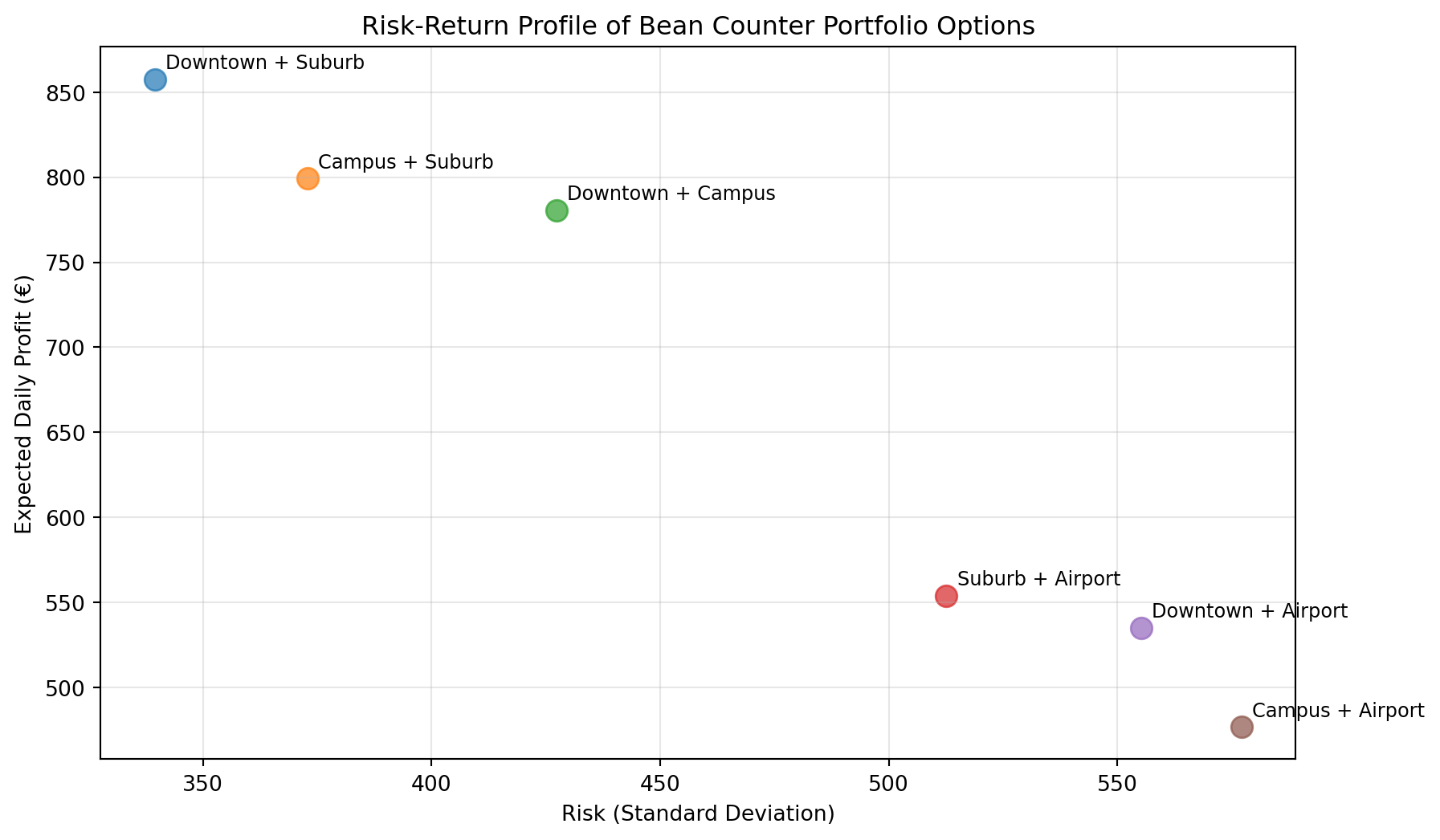
Exercise 4.1 - Analyze All Portfolio Combinations
Bean Counter can afford to open exactly 2 new locations. Which pair should they choose for maximum profitability?
# Analyze all possible pairs of locations# Get all combinations of 2 locationslocation_names =list(locations.keys())pairs =list(combinations(location_names, 2))# YOUR CODE BELOW# Analyze each portfolioportfolio_results = []for pair in pairs:# Get profits for each location in the pair profits_1 = location_profits[pair[0]] profits_2 = location_profits[pair[1]]# Portfolio assumes you open two locations portfolio_profit =# Your task!# Calculate metrics result = {'pair': f"{pair[0]} + {pair[1]}",'mean': , # Your task!'std': , # Your task!'prob_loss': , # Your task!'var_5': # Your task! } portfolio_results.append(result)# Convert to DataFrame and sort by mean profitdf_portfolios = pd.DataFrame(portfolio_results)df_portfolios = df_portfolios.sort_values('mean', ascending=False)# Find best portfolio by mean return (include only the variable name and the value!)best_mean_portfolio =# Your task!best_mean_value =# Your task!
Code
# Don't modify belowassertlen(portfolio_results) ==6, "Should have 6 portfolio combinations"assert'Downtown + Suburb'in best_mean_portfolio or'Suburb + Downtown'in best_mean_portfolio, \f"Best mean portfolio should include Downtown + Suburb, got {best_mean_portfolio}"assert700< best_mean_value <900, f"Best mean should be ~800, got {best_mean_value:.2f}"print("Portfolio analysis correct!")print("\nAll Portfolio Combinations:")print(df_portfolios.to_string(index=False))
Section 5 - Making Strategic Recommendations
Now let’s visualize and make a final recommendation!
Based on your analysis, make a strategic expansion recommendation for Bean Counter.
# YOUR CODE BELOW# Which portfolio maximizes expected profit? (Only the name)max_profit_portfolio =# Which portfolio minimizes risk (lowest std)? (Only the name)min_risk_portfolio =# Your final recommendation (choose one)final_recommendation =# Choose the portfolio you would recommend
Code
# Don't modify belowassert final_recommendation in df_portfolios['pair'].values, "Must choose an actual portfolio"print(f"\nYour Recommendation: {final_recommendation}")
Conclusion
Outstanding work, CEO! You’ve successfully applied Monte Carlo simulation to Bean Counter’s expansion strategy and mastered the key skills needed for the TechVenture competition:
Simulating uncertain returns using probability distributions
Making data-driven recommendations with clear justification
When you tackle the TechVenture challenge, apply what you’ve learned at Bean Counter:
Start Simple: Get one startup simulation working first
Verify Distributions: Plot histograms to check your simulations
Calculate All Metrics: Don’t just look at mean returns
Compare Systematically: Analyze all 6 pairs
Justify Clearly: Explain WHY your choice is best
Key Differences for Competition
The competition uses:
Investment returns instead of daily profits
Different distributions (some normal, one uniform)
Larger scale (€1M investments vs daily operations)
But the approach is identical! Apply what you’ve learned here.
Just as you’ve optimized Bean Counter’s expansion, use scoring functions in the competition to make objective decisions when multiple factors matter. Your journey from Barista Trainee to CEO has prepared you for this!
Good luck in the TechVenture Investment Challenge, CEO!