Welcome back, CEO! After successfully using Monte Carlo simulation to plan Bean Counter’s expansion, you now face a new challenge: predicting future demand for your seasonal products.
The Seasonal Challenge: Bean Counter has expanded beyond regular coffee into seasonal drinks:
Iced Coffee (summer favorite)
Pumpkin Spice Latte (fall special)
Peppermint Hot Chocolate (winter warmer)
You have 2 years of daily sales data. The board wants accurate forecasts for next month to optimize inventory. Overstock means waste (drinks expire), understock means lost sales and unhappy customers!
NoteHow to Use This Tutorial
Cells marked with “YOUR CODE BELOW” expect you to write code. Test your solutions with the provided assertions. Work through the sections in order - each builds on previous concepts!
import numpy as npimport pandas as pdimport matplotlib.pyplot as pltfrom datetime import datetime, timedelta# Set random seed for reproducibilitynp.random.seed(2025)print("Libraries loaded! Time to predict Bean Counter's future.")
Libraries loaded! Time to predict Bean Counter's future.
Section 1 - Working with Time Series Data
Before we can forecast, we need to understand how to work with dates and time-based data in pandas.
Understanding Date Conversion
# Example: Converting strings to datesdate_strings = ['2024-01-15', '2024-02-20', '2024-03-10']dates = pd.to_datetime(date_strings)print("Original strings:", date_strings)print("\nConverted to datetime:", dates)print("\nExtract components:")print(f" Months: {dates.month.tolist()}")print(f" Day of week: {dates.day_name().tolist()}")
Original strings: ['2024-01-15', '2024-02-20', '2024-03-10']

Converted to datetime: DatetimeIndex(['2024-01-15', '2024-02-20', '2024-03-10'], dtype='datetime64[ns]', freq=None)

Extract components:
  Months: [1, 2, 3]
  Day of week: ['Monday', 'Tuesday', 'Sunday']
Use .dt accessor to extract date parts:
.dt.month - Month (1-12)
.dt.day_of_week - Day (0=Monday, 6=Sunday)
.dt.quarter - Quarter (1-4)
.dt.is_month_end - Boolean for month end
To access specific elements, e.g. the third month of a year from a DataFrame, you can use df['date'].dt.month.iloc[2]. Step by step this happens:
You access the date column using df['date'].
You use the .dt accessor to extract the month part.
You use .iloc[2] to select the third element.
Exercise 1.1 - Load and Prepare Sales Data
Create a DataFrame with Bean Counter’s sales data and convert the date column properly.
# DON'T CHANGE ANYTHING BELOW!# Creates sample sales data for Bean Counter (3 years for enough seasonal cycles)dates = pd.date_range(start='2022-01-01', end='2024-12-31', freq='D')# Generate sales with trend and seasonalitybase_sales =100trend = np.linspace(0, 60, len(dates)) # Growing trend over 3 years# Summer peaks for iced coffee! (high in June-Aug, low in Dec-Feb)seasonal =45* np.sin(2* np.pi * (np.arange(len(dates)) -80) /365.25) # Yearly pattern, peaks in summerweekly =15* np.sin(2* np.pi * np.arange(len(dates)) /7) # Weekend peaksnoise = np.random.normal(0, 20, len(dates)) # Controlled noisesales = base_sales + trend + seasonal + weekly + noise# DON'T CHANGE ANYTHING ABOVE!
NoteCreating DataFrames and Working with Dates
# Create DataFrame from dictionarydf = pd.DataFrame({'col1': values1, 'col2': values2})# Access datetime attributes with .dtdf['date'].dt.month # Extract month (1-12)df['date'].dt.year # Extract yeardf['date'].dt.day # Extract day# Get first/last elementdf['column'].iloc[0] # First elementdf['column'].iloc[-1] # Last element
# YOUR CODE BELOW# Create DataFrame with date and sales columnsdf =# Create the DataFrame with 'date' and 'sales' columns# Extract month from the date column# Hint: Use .dt.month to get month, then .iloc[0] or .iloc[-1]first_month =# Get the month of the first datelast_month =# Get the month of the last date
Code
# Don't modify below - these test your solutionassert'date'in df.columns, "DataFrame should have a 'date' column"assert'sales'in df.columns, "DataFrame should have a 'sales' column"assert first_month ==1, f"First month should be January (1), got {first_month}"assert last_month ==12, f"Last month should be December (12), got {last_month}"print("Great! Sales data loaded and dates properly formatted!")# Quick visualization of your loaded dataplt.figure(figsize=(12, 8))plt.plot(df['date'], df['sales'], linewidth=1, alpha=0.7, color='#537E8F')plt.xlabel('Date')plt.ylabel('Sales (drinks)')plt.title('Bean Counter Sales - Your Loaded Data')plt.grid(True, alpha=0.3)plt.tight_layout()plt.show()
Exercise 1.2 - Analyze Sales Patterns
Calculate key statistics about Bean Counter’s sales to understand the data.
You can use methods like mean(), max(), and min() to calculate basic statistics with DataFrames. You just need to call these methods on the ‘sales’ column of the DataFrame.
# YOUR CODE BELOW# Calculate basic statisticsmean_sales =# Average daily salesmax_sales =# Highest sales daymin_sales =# Lowest sales day
Code
# Don't modify belowassert115< mean_sales <135, f"Mean sales should be ~125, got {mean_sales:.1f}"assert max_sales >180, f"Max sales should be >180, got {max_sales:.1f}"assert min_sales <70, f"Min sales should be <70, got {min_sales:.1f}"print(f"Excellent! Analysis complete!")print(f"Daily average: {mean_sales:.0f} drinks")
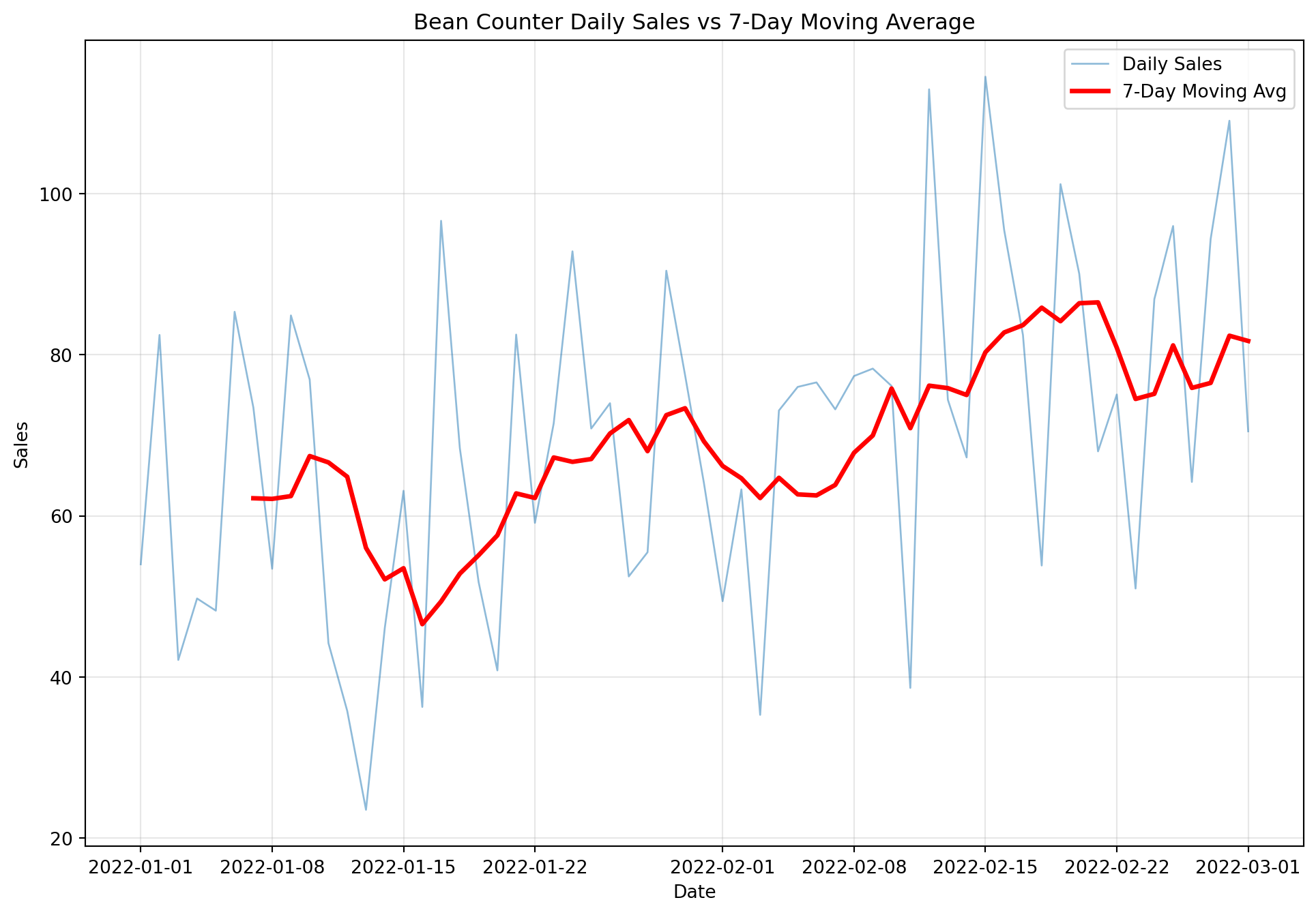
Section 2 - Moving Averages: Smoothing the Noise
Daily sales are noisy. Moving averages help us see the underlying patterns by averaging nearby data points.
Understanding Moving Averages
The Concept: A moving average smooths data by calculating the average of a “window” of recent values. As we move forward in time, the window slides along the data.
The first (window-1) values will be NaN because there aren’t enough previous values to calculate the average! For a 7-day MA, the first 6 values are NaN. To find the number of NaN values in a moving average, you can use the isna() method to check for NaN values and then count them using the sum() method, e.g., df['MA7'].isna().sum().
Exercise 2.1 - Create Multiple Moving Averages
Calculate different window sizes to see their smoothing effects.
NoteRolling Windows and NaN Values
# Create rolling window and calculate meandf['MA7'] = df['sales'].rolling(window=7).mean()# Count missing (NaN) valuesna_count = df['MA7'].isna().sum()# Why NaN? First 6 rows have no 7-day window yet!# Window of 7 → first 6 values are NaN
# YOUR CODE BELOW# Calculate moving averages with different windowsdf['MA3'] =# 3-day moving averagedf['MA14'] =# 14-day (2 week) moving averagedf['MA30'] =# 30-day (monthly) moving average# Count NaN values in each# Hint: Use .isna().sum()na_count_3 =# Number of NaN values in MA3na_count_14 =# Number of NaN values in MA14na_count_30 =# Number of NaN values in MA30
Code
# Don't modify belowassert na_count_3 ==2, f"MA3 should have 2 NaN values, got {na_count_3}"assert na_count_14 ==13, f"MA14 should have 13 NaN values, got {na_count_14}"assert na_count_30 ==29, f"MA30 should have 29 NaN values, got {na_count_30}"assert df['MA30'].std() < df['MA3'].std(), "MA30 should be smoother (lower std) than MA3"print("Perfect! Moving averages calculated correctly!")print(f" MA30 is {df['MA3'].std() / df['MA30'].std():.1f}x smoother than MA3")# Visualize the smoothing effectplt.figure(figsize=(12, 8))plt.plot(df['date'], df['sales'], linewidth=1, alpha=0.2, color='gray', label='Daily Sales')plt.plot(df['date'], df['MA3'], linewidth=2, alpha=0.3, color='#DB6B6B', label='MA3 (noisy)')plt.plot(df['date'], df['MA14'], linewidth=2, alpha=0.6, color='#537E8F', label='MA14 (balanced)')plt.plot(df['date'], df['MA30'], linewidth=2.5, alpha=0.9, color='#F6B265', label='MA30 (smooth)')plt.xlabel('Date')plt.ylabel('Sales (drinks)')plt.title('Comparing Moving Average Windows - Notice How MA30 is Smoothest')plt.legend(loc='best')plt.grid(True, alpha=0.3)plt.tight_layout()plt.show()
Exercise 2.2 - Weighted Moving Average
Recent data often matters more! A weighted moving average assigns higher weights to recent observations.
The Idea: Instead of equal weights [1/7, 1/7, 1/7, 1/7, 1/7, 1/7, 1/7], we use custom weights like [0.05, 0.05, 0.10, 0.15, 0.20, 0.20, 0.25] where recent days get more importance.
# YOUR CODE BELOW# Create weighted moving average (last 7 days)# Weights: [0.05, 0.05, 0.10, 0.15, 0.20, 0.20, 0.25] (sum = 1.0)weights = np.array([0.05, 0.05, 0.10, 0.15, 0.20, 0.20, 0.25])# Calculate WMA for day 30 (using days 24-30)sales_window = df['sales'].iloc[24:31].values # Days 24-30 (7 days)wma_day30 =# Calculate weighted average: np.sum(sales * weights)# Compare to simple average for same windowsma_day30 =# Simple average: np.mean(sales_window)
Code
# Don't modify belowassert50< wma_day30 <150, f"WMA should be between 50-150, got {wma_day30:.1f}"assertabs(wma_day30 - sma_day30) <20, "WMA and SMA shouldn't differ by more than 20"assertlen(weights) ==7, "Should have 7 weights"assertabs(sum(weights) -1.0) <0.01, "Weights should sum to 1.0"print(f"✓ Excellent! Weighted MA: {wma_day30:.1f}, Simple MA: {sma_day30:.1f}")
Section 3 - Simple Forecasting Methods
Now let’s build actual forecasting functions! We’ll start with simple methods before moving to more advanced techniques.
Building Basic Forecast Functions
def naive_forecast(data, periods=1):"""Naive forecast: tomorrow = today (simplest baseline)"""return [data.iloc[-1]] * periodsdef moving_average_forecast(data, window=7, periods=1):"""Forecast using moving average of last 'window' days""" ma = data.iloc[-window:].mean()return [ma] * periods# Example usageprint(f"Last value: {df['sales'].iloc[-1]:.1f}")print(f"Naive forecast (next 3 days): {naive_forecast(df['sales'], 3)}")print(f"MA forecast (next 3 days): {moving_average_forecast(df['sales'], 7, 3)}")
Last value: 110.3
Naive forecast (next 3 days): [np.float64(110.26466239914413), np.float64(110.26466239914413), np.float64(110.26466239914413)]
MA forecast (next 3 days): [np.float64(117.69909865143963), np.float64(117.69909865143963), np.float64(117.69909865143963)]
Understanding Exponential Smoothing
The Problem with Simple MA: All days in the window are treated equally. The sale from 7 days ago has the same importance as yesterday.
Exponential Smoothing Solution: Weight recent observations more heavily, and the weight decreases exponentially as you go back in time.
The Formula:\[\text{Forecast}_{t+1} = \alpha \times \text{Actual}_t + (1-\alpha) \times \text{Forecast}_t\]
Where α (alpha) is between 0 and 1:
α = 0.9: Very responsive (trust recent data heavily)
α = 0.3: Balanced (typical default)
α = 0.1: Very stable (smooth out noise)
You can also forecast multiple periods at once. The result is then just the last value of the forecast for all future periods.
Exercise 3.1 - Implement Exponential Smoothing
Create an exponential smoothing forecast function.
TipExponential Smoothing Formula
Core idea: New forecast = mix of (actual data) and (old forecast)
# Access last elementlast_value = my_list[-1]# Multiply a list (creates repeated elements)future = [100] *3# [100, 100, 100]# In a loop, use data.iloc[i] to get value at index ifor i inrange(1, len(data)): current_value = data.iloc[i]
# YOUR CODE BELOWdef exponential_smoothing_forecast(data, alpha=0.3, periods=1):""" Exponential smoothing forecast Formula: forecast = alpha * latest_value + (1-alpha) * previous_forecast For first forecast, use the first actual value """ forecasts = [data.iloc[0]] # Start with first value# Calculate smoothed values for historical datafor i inrange(1, len(data)):# Apply exponential smoothing formula# Hint: data.iloc[i] is current actual, forecasts[-1] is previous forecast forecast =# alpha * current_actual + (1-alpha) * previous_forecast forecasts.append(forecast)# Use last smoothed value for future periods last_forecast = forecasts[-1] future =# Return list: [last_forecast] * periodsreturn future# Test your functiontest_data = pd.Series([100, 105, 98, 103, 107])result = exponential_smoothing_forecast(test_data, alpha=0.3, periods=2)
Code
# Don't modify belowassertlen(result) ==2, "Should return 2 forecasts"assert100< result[0] <105, f"Forecast should be between 100-105, got {result[0]:.1f}"assert result[0] == result[1], "All future periods should have same forecast"print(f"✓ Great! Exponential smoothing implemented correctly!")print(f" Forecast: {result[0]:.1f} for next 2 periods")
Section 4 - Advanced Methods: Holt’s Method
The Problem: Simple exponential smoothing assumes data is flat (no trend). But Bean Counter is growing! Sales are trending upward.
Holt’s Method Solution: Track TWO things separately:
Level - Where are we right now?
Trend - How fast are we growing per period?
Understanding Time Series Aggregation
Before applying Holt’s method, we need to learn how to convert daily data to weekly data using resample().
Forecast = Current level + (periods ahead × trend)
Let’s see Holt’s method in action using Python’s statsmodels library:
from statsmodels.tsa.holtwinters import ExponentialSmoothing# Create sample trending dataweeks = pd.date_range('2024-01-01', periods=20, freq='W')trending_sales =100+3*np.arange(20) + np.random.normal(0, 5, 20)ts_trending = pd.Series(trending_sales, index=weeks)# Fit Holt's model (trend, but no seasonality)model_holt = ExponentialSmoothing(ts_trending, trend='add', seasonal=None)fitted_holt = model_holt.fit(smoothing_level=0.3, smoothing_trend=0.2)# Forecast next 4 periodsforecast_holt = fitted_holt.forecast(steps=4)print("Last 3 actual values:")print(ts_trending.tail(3))print(f"\nNext 4 week forecast with Holt's method:")print(forecast_holt)print("\nNotice: Forecasts increase each week (captures trend!)")
Last 3 actual values:
2024-05-05    147.700470
2024-05-12    156.602208
2024-05-19    165.404895
Freq: W-SUN, dtype: float64

Next 4 week forecast with Holt's method:
2024-05-26    161.150728
2024-06-02    164.553567
2024-06-09    167.956406
2024-06-16    171.359244
Freq: W-SUN, dtype: float64

Notice: Forecasts increase each week (captures trend!)
Exercise 4.1 - Apply Holt’s Method to Bean Counter
Bean Counter’s sales are growing. Use Holt’s method to capture this trend.
# Prepare weekly data (aggregate daily to weekly to reduce noise)df_weekly = df.set_index('date').resample('W')['sales'].mean()# YOUR CODE BELOW# Split: first 90 weeks for training, last 14 for testingtrain_weekly =# First 90 weekstest_weekly =# Last 14 weeks# Fit Holt's modelmodel_holt =# ExponentialSmoothing with trend='add', seasonal=Nonefitted_holt =# Fit the modelholt_forecast =# Forecast 14 weeks
You have ideally 2 full seasonal cycles (e.g., 2 years for yearly patterns)
Let’s demonstrate with monthly data:
# Create data with trend AND seasonalitymonths = pd.date_range('2022-01-01', periods=24, freq='M')trend_comp = np.linspace(100, 150, 24)seasonal_comp =30* np.sin(2* np.pi * np.arange(24) /12)monthly_sales = trend_comp + seasonal_comp + np.random.normal(0, 5, 24)ts_seasonal = pd.Series(monthly_sales, index=months)# Fit Holt-Winters modelmodel_hw = ExponentialSmoothing( ts_seasonal, trend='add', # Additive trend seasonal='add', # Additive seasonality seasonal_periods=12# 12 months = 1 year)fitted_hw = model_hw.fit()# Forecast next 6 monthsforecast_hw = fitted_hw.forecast(steps=6)print("Last 3 months actual:")print(ts_seasonal.tail(3))print(f"\nNext 6 months forecast:")print(forecast_hw)print("\nNotice: Seasonal pattern continues (Jan is low, summer will be high)")
Last 3 months actual:
2023-10-31    121.824928
2023-11-30    121.818264
2023-12-31    134.481744
Freq: ME, dtype: float64

Next 6 months forecast:
2024-01-31    157.483905
2024-02-29    175.816373
2024-03-31    184.848236
2024-04-30    187.735748
2024-05-31    181.651676
2024-06-30    183.597933
Freq: ME, dtype: float64

Notice: Seasonal pattern continues (Jan is low, summer will be high)
/var/folders/_5/jkkjxxdd5f1955l380dky7n80000gn/T/ipykernel_96555/3645223708.py:2: FutureWarning: 'M' is deprecated and will be removed in a future version, please use 'ME' instead.
  months = pd.date_range('2022-01-01', periods=24, freq='M')
Exercise 5.1 - Apply Holt-Winters
Now use Holt-Winters to capture both trend and seasonality in Bean Counter’s weekly sales.
Note: For weekly data with yearly seasonality, we need 2+ years (104+ weeks). We’ll use quarterly seasonality (13 weeks) since we have 104 weeks total.
# YOUR CODE BELOW# Use the weekly data we created earlier# Split: first 150 weeks training, last 8 weeks testingtrain_hw = df_weekly.iloc[:150]test_hw = df_weekly.iloc[150:158] # Exactly 8 weeks for testing (all remaining data)# Fit Holt-Winters with yearly seasonality (52 weeks = 1 year)model_hw =# ExponentialSmoothing with trend='add', seasonal='add', seasonal_periods=52fitted_hw =# Fit the modelhw_forecast =# Forecast 8 weeks# Compare all three methods on same test periodsimple_forecast = exponential_smoothing_forecast(train_hw, alpha=0.3, periods=8)holt_forecast_test = ExponentialSmoothing(train_hw, trend='add', seasonal=None).fit().forecast(8)
Code
# Don't modify belowassertlen(hw_forecast) ==8, "Should forecast 8 weeks"# Holt-Winters should vary (seasonality), simple ES should be flathw_variation = hw_forecast.std()simple_variation = np.std(simple_forecast)assert hw_variation > simple_variation, "Holt-Winters should show more variation (seasonality)"print(f"Fantastic! Holt-Winters applied successfully!")print(f"Holt-Winters range: {hw_forecast.min():.1f} to {hw_forecast.max():.1f}")print(f"Simple ES (flat): {simple_forecast[0]:.1f}")
Section 6 - Measuring Forecast Accuracy
How good are our forecasts? Let’s measure and compare!
MAE: 2.0 (average error)
RMSE: 2.0 (penalizes big errors)
TipMAE vs RMSE
MAE: Average error size (easier to interpret, in same units as data)
RMSE: Penalizes large errors more heavily (sensitive to outliers)
In business: MAE often preferred for its simplicity and interpretability
Exercise 6.1 - Compare All Methods
Let’s have a forecasting comparison! Which method works best for Bean Counter?
# YOUR CODE BELOW# Calculate MAE for all methods on the test period (last 8 weeks)test_actual = test_hw.values# Convert forecasts to numpy arrays for comparisonsimple_array = np.array(simple_forecast)holt_array = holt_forecast_test.valueshw_array = hw_forecast.values# Calculate MAE for each methodmae_simple =# MAE for simple exponential smoothingmae_holt =# MAE for Holt's methodmae_hw =# MAE for Holt-Winters# Find the winner (lowest MAE)mae_values = [mae_simple, mae_holt, mae_hw]best_method_index = np.argmin(mae_values) # Index of best method