Introduction to Metaheuristics

Lecture 9 - Management Science

Author

Dr. Tobias Vlćek

Introduction

Client Briefing: La Étoile

. . .

Restaurant Manager’s Crisis:

“I need to schedule my 18 servers across 6 shifts this weekend. Shifts have different lengths (4-6 hours), and if I don’t have enough experienced servers on busy shifts, we face penalties per missing experienced server from our parent company!”

The Staffing Challenge

A restaurant facing a weekend scheduling crisis:

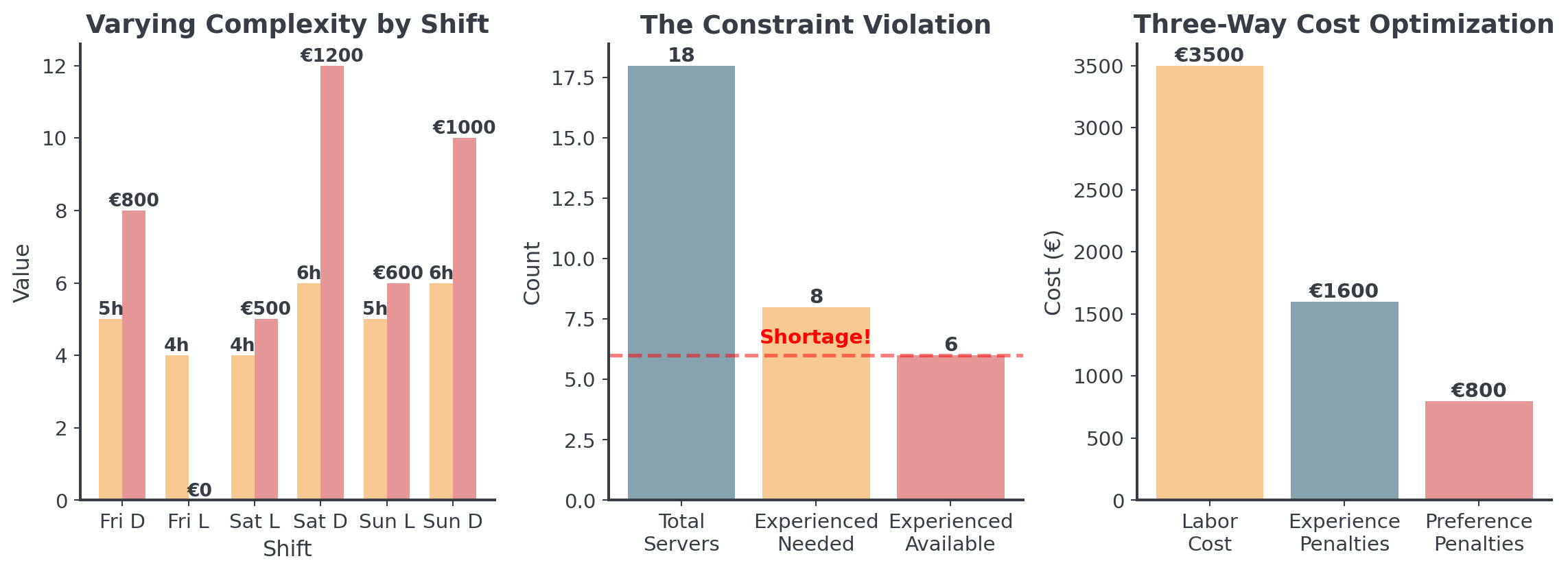
La Étoile’s Problem:

18 servers available (6 experienced @ €75/hr, 12 junior @ €25/hr)
6 shifts with varying lengths (4-6 hours each)
Each shift needs 3 servers (at least 1 experienced)
Server preferences matter (1-10 scale, affects quality)

. . .

Question: How to balance labor costs, penalties, AND staff?

The Cost Impact: Why This Matters

The financial stakes are significant with these large penalties:

Minimum Labor Cost: ~€3,500 (everyone works once)
Experience Penalties: €0-€1,200 per missing experienced server
Preference Penalties: €0-€180 per unhappy assignment
Worst Case: Over €9,000 if poorly scheduled!
Best Case: ??? with smart optimization

. . .

Potentially up to large difference between good and bad scheduling!

Restaurant Staffing: The Numbers

The real-world complexity we’re dealing with:

. . .

With varying shifts, preferences, and penalties, this is will be a real challenge!

Today’s Objectives

What you’ll understand after this lecture:

Why local search fails: Recap on the local optima trap
Escape mechanisms: How to accept worse solutions strategically
Four powerful metaheuristics: SA, GA, Tabu Search, ACO
Selection criteria: When to use which algorithm

Hiking in Fog

Remember the metaphor with blindfolded eyes from last lecture?

Goal: Find the highest peak in a mountain range
Challenge: You’re hiking in thick fog (can only see 10 meters)
Position: Your X,Y coordinates = your decisions
Altitude: Your current solution quality
Problem: You might climb a small hill and think it’s the summit!

. . .

This metaphor will guide us through all metaheuristics today!

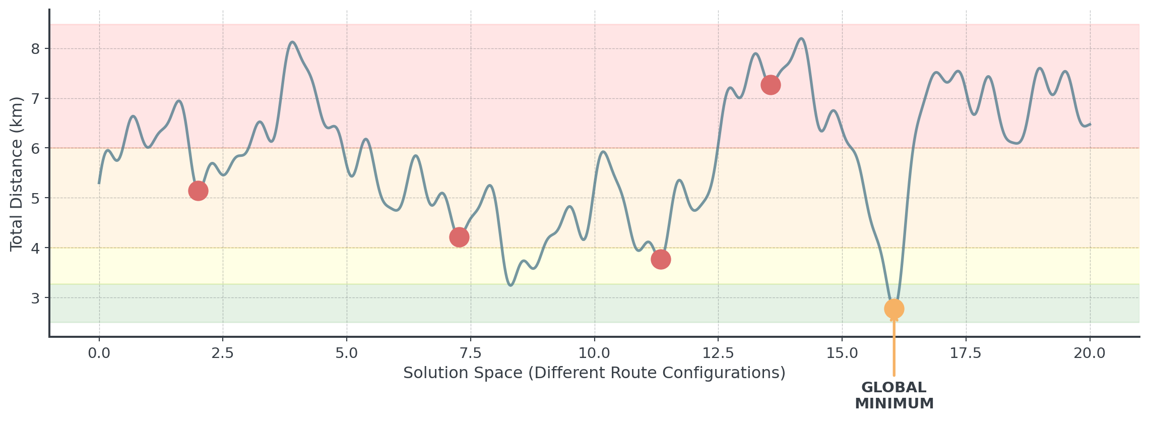
Recap: Local Optima

Real problems often have thousands of local optima!

. . .

Question: Any idea how to escape local optima?

Why Simple Methods Fail

The Silo Problem

Why neighborhood optimization fails:

Technical View: Local Optima

Algorithm climbs nearest hill
Gets stuck on “foothill”
Can’t see the mountain beyond
Every move looks worse
Believes it found the best

Analogy: Department Silos

Sales optimizes sales metrics
Engineering optimizes quality
Finance optimizes costs
Each department “wins”
Company performance loses!

. . .

Sum of local bests ≠ Global best

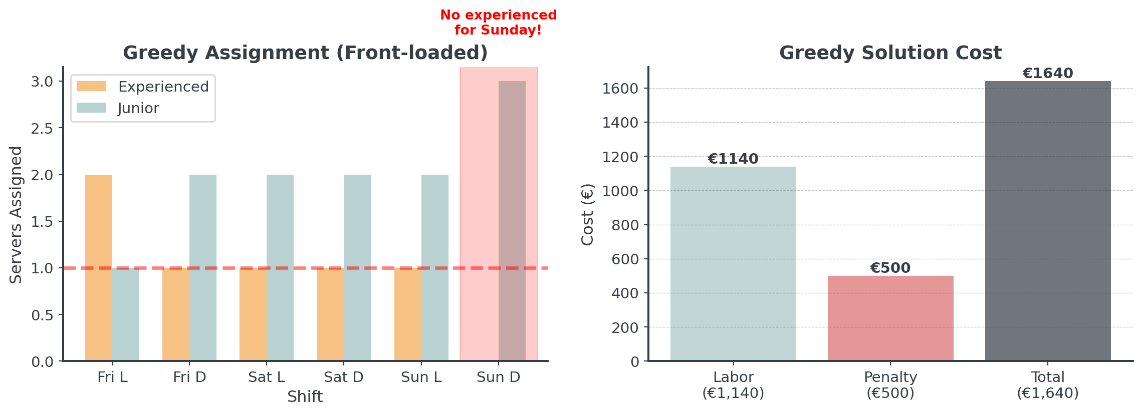
Why Greedy Gets Stuck

Greedy algorithms can simply trap themselves:

. . .

. . .

Greedy allocates resources early, creating problems later!

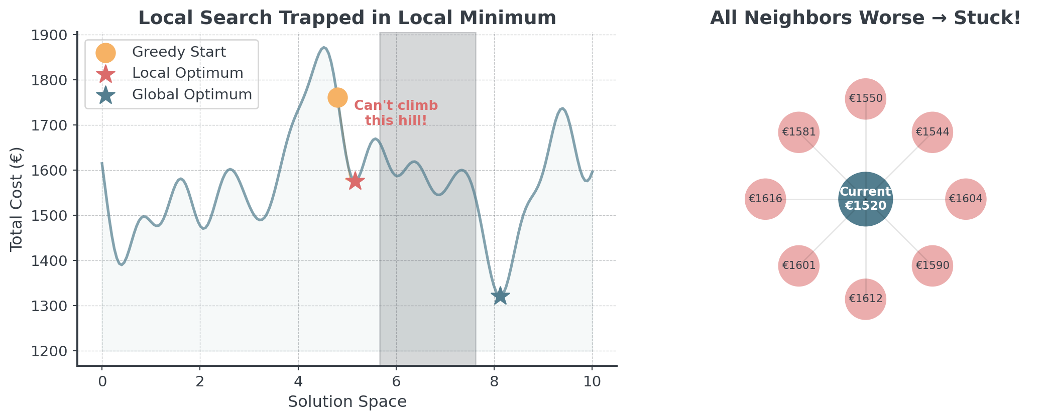
Local Search Also Struggles

Because we only ever accept better solutions during search:

. . .

. . .

Question: What can we do to cope with this situation?

Metaheuristic #1: Simulated Annealing

Core Concepts

The fundamental components:

Solution = One complete schedule/route/plan
Neighbor = A slightly modified version
Cost = How good/bad the solution is

. . .

The Strategy

Always accept improvements
Sometimes accept worse solutions (the change!)

. . .

Think of it as strategic risk-taking that decreases over time!

The Metallurgy Metaphor

How annealing steel inspired an optimization algorithm:

Annealing Metal:

Heat to high temperature
Atoms move freely
Slowly cool down
Forms crystal structure

Optimization:

Start with high “temperature”
Accept bad moves often
Gradually reduce temperature
Converge to good solution

. . .

The willingness to temporarily accept worse solutions is what enables finding the summit!

Temperature Controls Acceptance

Probability of accepting worse solutions lowers with temp:

. . .

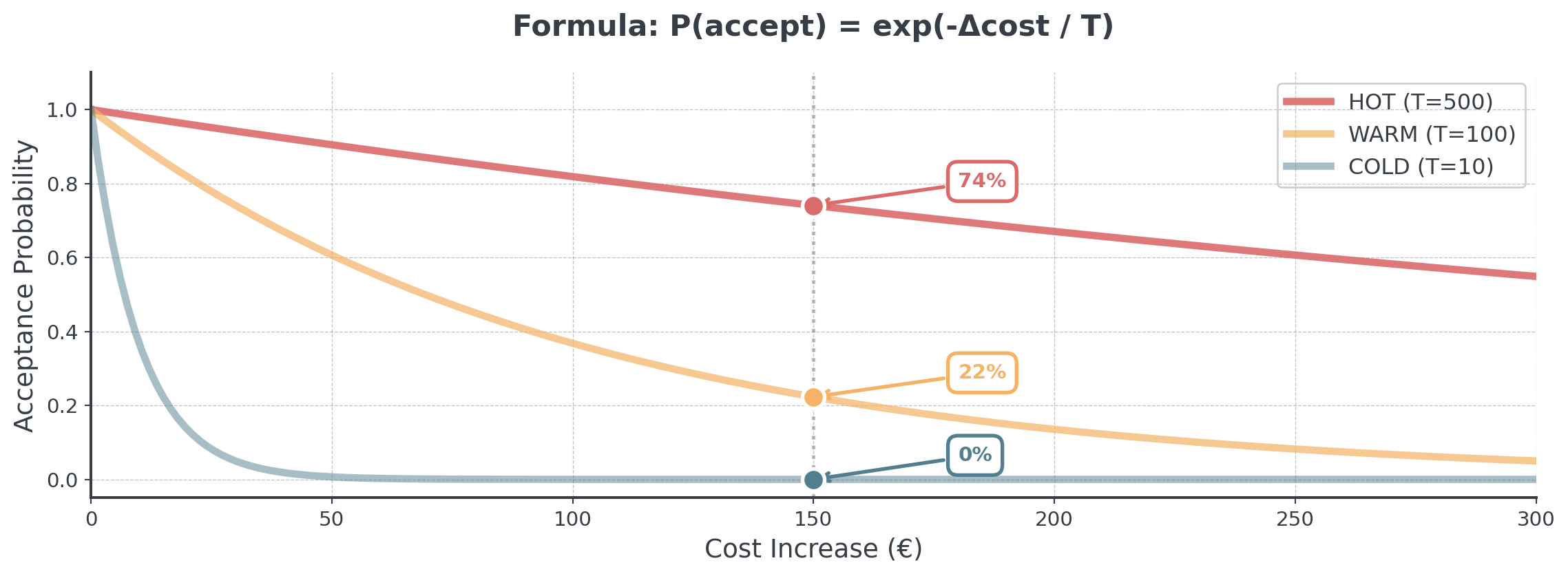
We essentially compare the cost of the new schedule to the current cost and decide whether to accept the change based on the temperature and the difference in cost.

Concept

How Simulated Annealing Works (Pseudocode)

def simulated_annealing_concept(current_schedule):
    temperature = 500  # Start "hot" (adventurous)
    best_schedule = current_schedule
    
    while temperature > 1:
        # Step 1: Try a random change (like swapping two shifts)
        new_schedule = make_random_change(current_schedule)
        
        # Step 2: Is it better?
        if cost(new_schedule) < cost(current_schedule):
            current_schedule = new_schedule  # Always accept improvements
        else:
            # NEW: Sometimes accept worse solutions!
            # Hot temperature = more likely to accept
            # Cold temperature = less likely to accept
            if random() < acceptance_probability(temperature):
                current_schedule = new_schedule  # Accept anyway!
        
        # Step 3: Cool down (become less adventurous)
        temperature = temperature * 0.95
        
        # Remember the best we've ever seen
        if cost(current_schedule) < cost(best_schedule):
            best_schedule = current_schedule
    
    return best_schedule

SA in Action: Restaurant Staffing

A simplified weekend scheduling problem we’ll use throughout:

# SIMPLIFIED PROBLEM (used across ALL metaheuristics today)
"""
La Étoile's Weekend Challenge:
- 12 servers: 4 experienced (E1-E4), 8 junior (J1-J8)
- 6 shifts: Need 2 servers each
- Everyone works exactly 1 shift
"""

. . .

The initial greedy schedule has the following results:

. . .

Greedy Schedule Cost: €5,240
  Labor: €2250, Penalties: €1700, Unhappiness: €1290

. . .

Let’s see how Simulated Annealing can improve the solution!

Visualizing SA Performance

How temperature affects the search behavior:

. . .

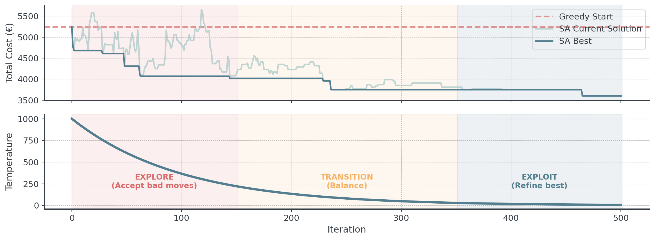
See how SA accepts worse solutions early, enabling escape from local optima!

Common SA Mistakes

Avoid these common implementation errors:

. . .

Mistake #1: Starting Too Cold

If temperature is too low → Acts like greedy (no exploration)
Fix: Start hot enough to accept bad moves

. . .

Mistake #2: Cooling Too Quickly

If you cool fast → Get stuck early
Fix: Cool slowly (multiply by 0.95-0.99, not 0.5)

. . .

Quick cooling is tempting for speed, but defeats the purpose of SA!

Temperature Parameter Impact

. . .

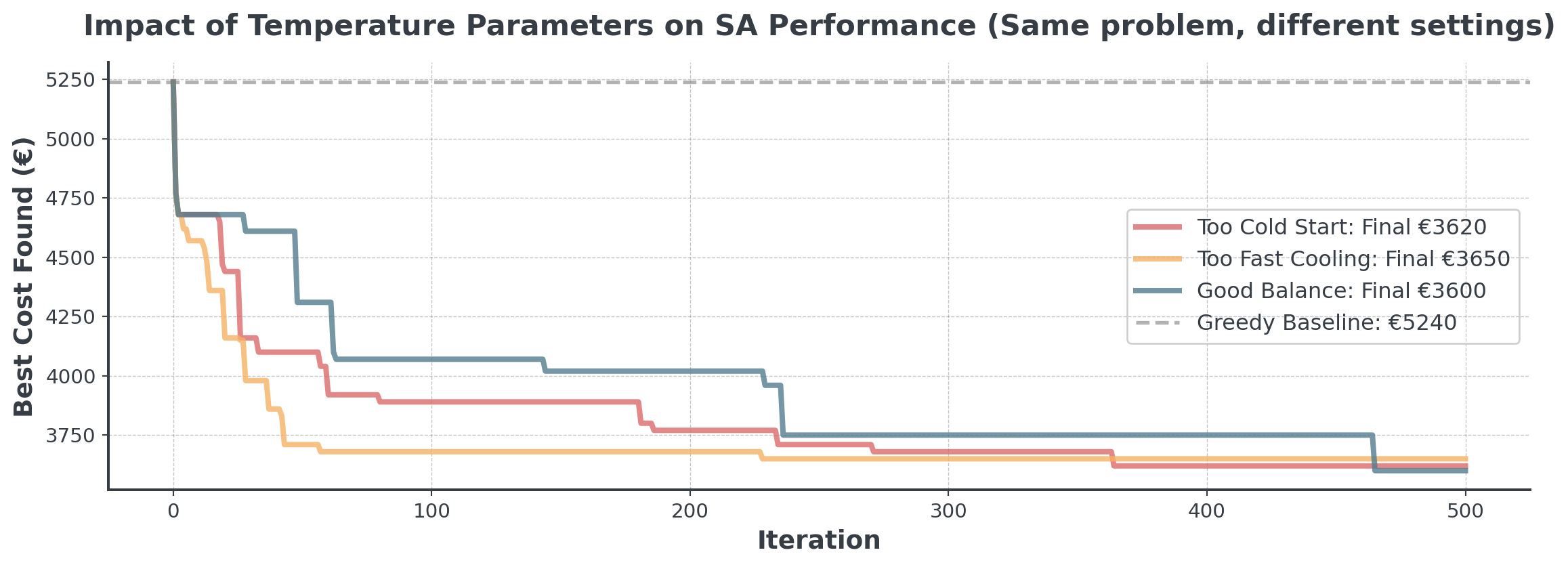
The “Good Balance” explores widely early, then refines carefully. Often you need to balance exploration and exploitation by experimenting with different parameters.

Metaheuristic #2: Genetic Algorithms

Evolution as Optimization

How natural selection inspires computational optimization:

Natural Selection:

Population of individuals
Fittest survive & reproduce
Offspring inherit traits
Mutations create diversity
Evolution finds adaptation

Optimization:

Population of solutions
Best solutions selected
Crossover combines solutions
Mutation adds variation
Evolution finds optimum

. . .

Just like successful products get more market share, better solutions get more “offspring” in the next generation. It’s survival of the fittest, but for schedules, routes, or designs!

The Genetic Process

Four stages repeat each generation:

Selection: Choose parents based on fitness
Crossover: Combine to create children
Mutation: Randomly modify children
Replacement: New generation replaces old
Population Evolution: Improve population quality

. . .

Let’s see each stage in detail with our restaurant problem!

Stage 1: Selection (Tournament)

How to choose which schedules get to “reproduce”:

. . .

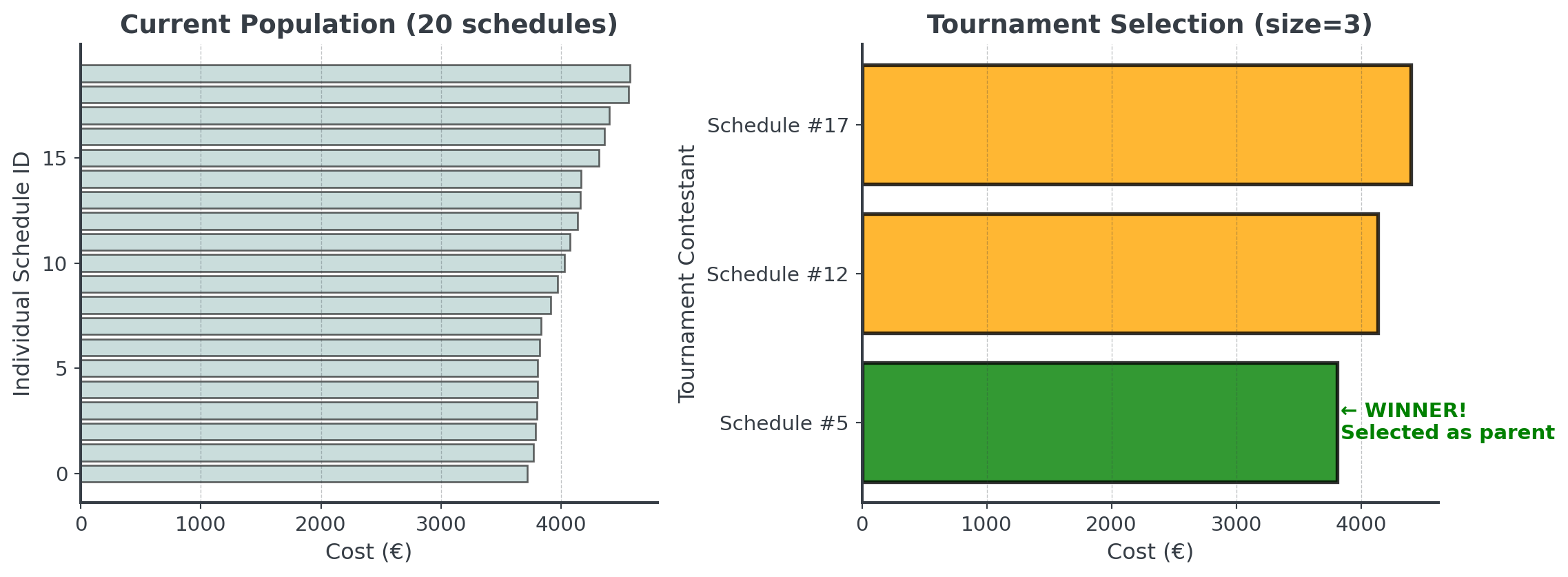
Each tournament selects one parent, then we pair them up sequentially for crossover.

Stage 2: Crossover (Recombination)

Combine two parent schedules to create offspring:

. . .

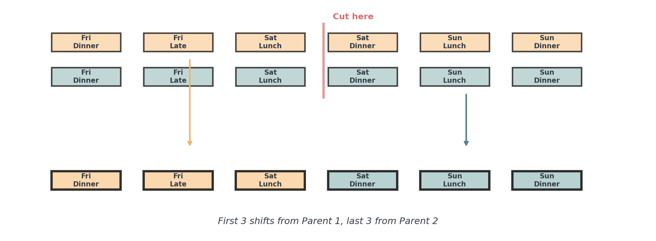
Crossover randomly combines good building blocks from both parents!

Stage 3: Mutation

Random changes maintain diversity and explore new solutions:

. . .

Mutation adds random exploration, like trying something completely new occasionally!

Stage 4: Replacement I

How do offspring join the population?

Generational: Replace entire population with offspring
Steady-State: Replace only worst individuals
Elitism: Always keep the best solutions

. . .

Our approach: Generational with Elitism, we create 20 offspring via repeated selection/crossover/mutation, but preserve the 2 best from current generation.

Stage 4: Replacement II

. . .

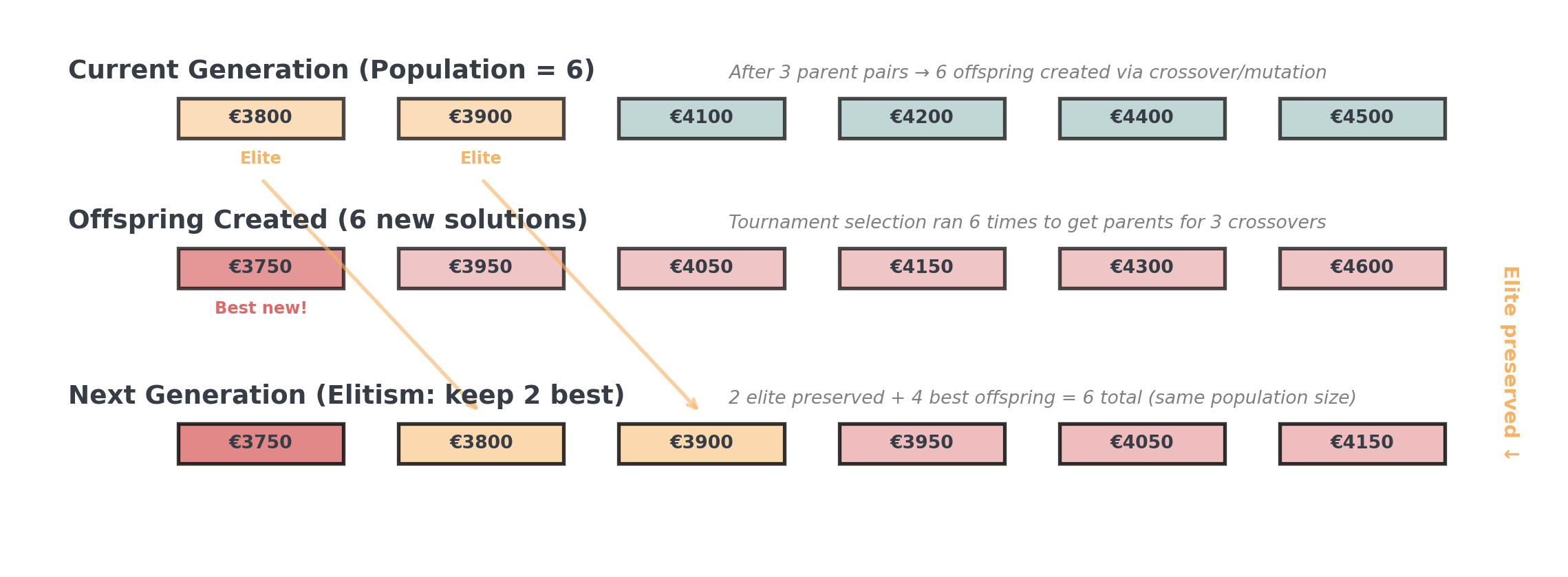
Elitism ensures we never lose our best solutions while exploring new ones!

Stage 5. Population Evolution

How the population improves over generations:

. . .

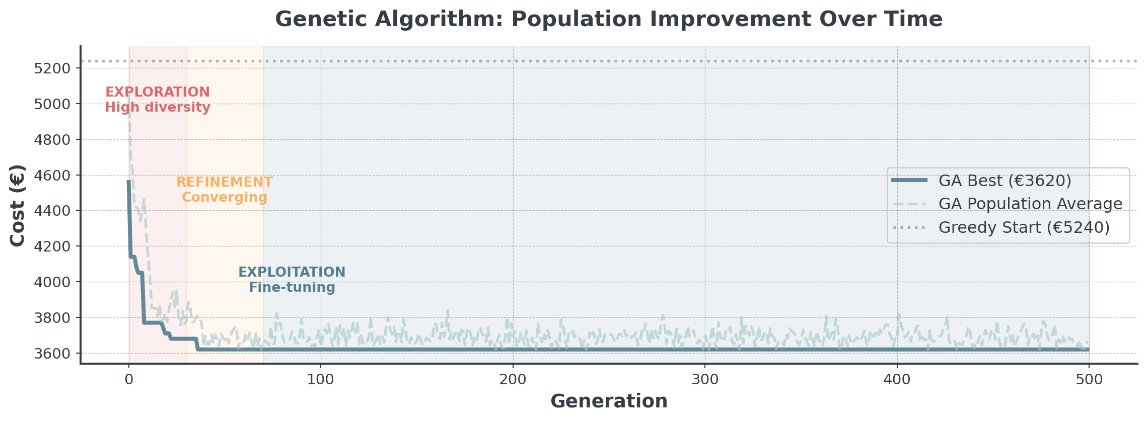
Notice how population average also improves (not just the best)!

GA vs SA: Head-to-Head

Comparing exploration strategies on the restaurant problem:

. . .

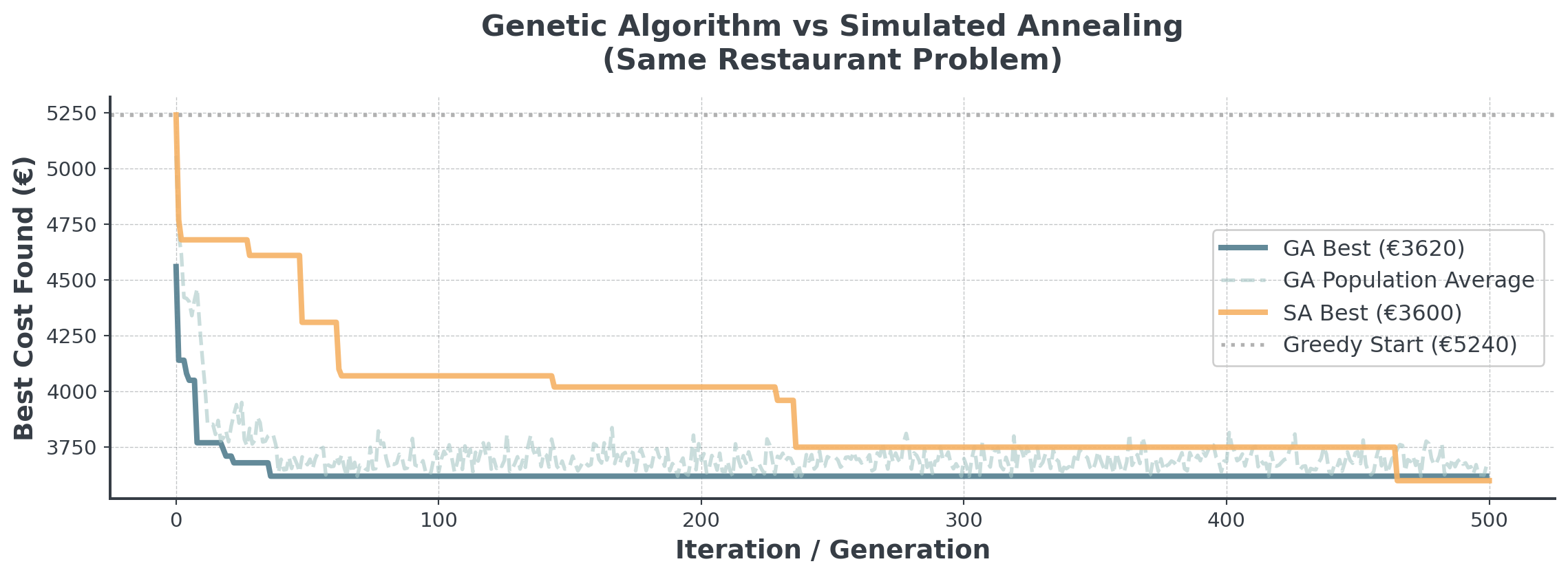
GA maintains population diversity, SA explores single solution path!

GA Mistakes: Population Issues

Avoid these population-related errors:

. . .

Mistake #1: Everyone Becomes Identical

If all solutions look the same → Lost diversity
Fix: More mutation, bigger population, tournament selection

. . .

Mistake #2: Too Greedy in Selection

Only keeping the very best → Premature convergence
Fix: Keep some variety, even if not perfect (elitism of 10-20%)

GA Mistakes: Implementation

Technical pitfalls to watch out for:

. . .

Mistake #3: Breaking the Rules

Crossover might create invalid schedules
Fix: Always check and repair after crossover/mutation

. . .

Mistake #4: Evolution Too Slow

Population too large or too many generations
Fix: Start small (50-100), tune based on convergence

Metaheuristic #3: Tabu Search

Core Idea

Using memory to avoid cycling through bad solutions:

Analogy:

Keep a list of recent dates
“Not going back there!”
Forces you to meet new people
After time, memory fades

In Optimization:

Recent solutions = “tabu”
Don’t revisit same schedules
Forces exploration of new areas
Tabu list has limited size

. . .

Like keeping “lessons learned”, you remember not to use them again, but after a while, you might reconsider!

Concept

How Tabu Search Works (Pseudocode)

def tabu_search_concept():
    tabu_list = []  # Our "never again" list
    current_solution = initial_schedule
    best_solution = current_solution
    
    while not done:
        # Look at all possible moves
        possible_moves = get_all_neighbor_moves(current_solution)
        
        # Filter out the "forbidden" moves
        allowed_moves = []
        for move in possible_moves:
            if move not in tabu_list:  # Not forbidden
                allowed_moves.append(move)
        
        # Pick the best allowed move (even if worse!)
        best_move = select_best(allowed_moves)
        current_solution = apply(best_move)
        
        # Update best if improved
        if cost(current_solution) < cost(best_solution):
            best_solution = current_solution
        
        # Remember this move (add to tabu list)
        tabu_list.append(best_move)
        if len(tabu_list) > 10:  # Keep list size manageable
            tabu_list.pop(0)  # Forget oldest
    
    return best_solution

Tabu Search on Restaurant Problem

Real implementation with memory-based exploration:

. . .

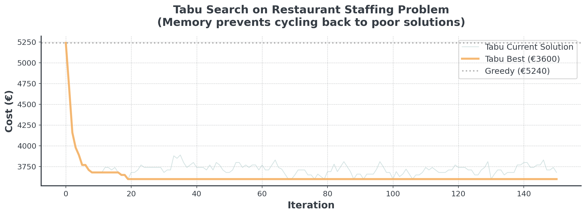
Tabu Search’s memory prevents revisiting bad solutions!

Metaheuristic #4: Ant Colony Optimization

The Core Idea

Collective intelligence through chemical signals:

Reviews:

Popular choices get more 5-star reviews
More reviews → more visibility
But old reviews fade over time
New patterns can emerge

In Optimization:

Good assignments get “pheromones”
Stronger choosen more likely
Evaporation against stagnation
Colony finds patterns

Imagine each server-shift pairing has a “rating” that increases when it works well in a schedule. Over time, the best pairings naturally get chosen more often!

How ACO Works on Scheduling

Four key stages in each iteration:

Construction: Each ant builds a schedule probabilistically
Evaluation & Evaporation: Measure quality, then fade all pheromones
Reinforcement: Good schedules deposit pheromones
Evolution: Repeat until colony converges

. . .

Let’s see each stage visually!

ACO: Key Parameters

Two critical parameters control the balance:

Evaporation Rate (ρ)

Higher ρ → More forgetting
Lower ρ → Stronger memory
Typical: 0.1 - 0.5
Too high: Colony never learns
Too low: Gets stuck early

Number of Ants

More ants → More exploration
Fewer ants → Faster iterations
Typical: 10 - 50
Too many: Slow, redundant
Too few: Miss good patterns

. . .

Start with ρ=0.3 and n_ants=20, then tune based on problem size.

Stage 1: Pheromone Construction

Ants don’t pick randomly, they follow the chemical trails

. . .

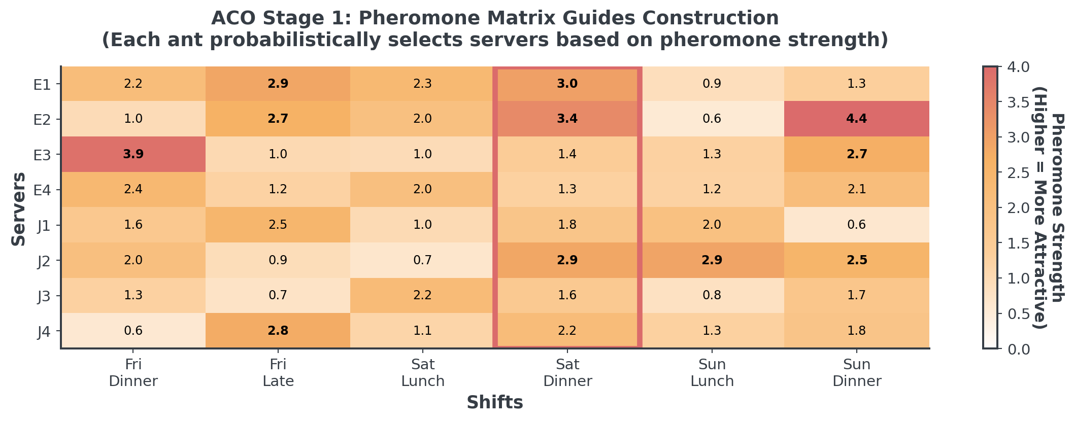
To build the initial pheromone matrix, each cell is initialized with a small positive value.

Stage 2: Evaluation & Evaporation

After all ants build schedules:

. . .

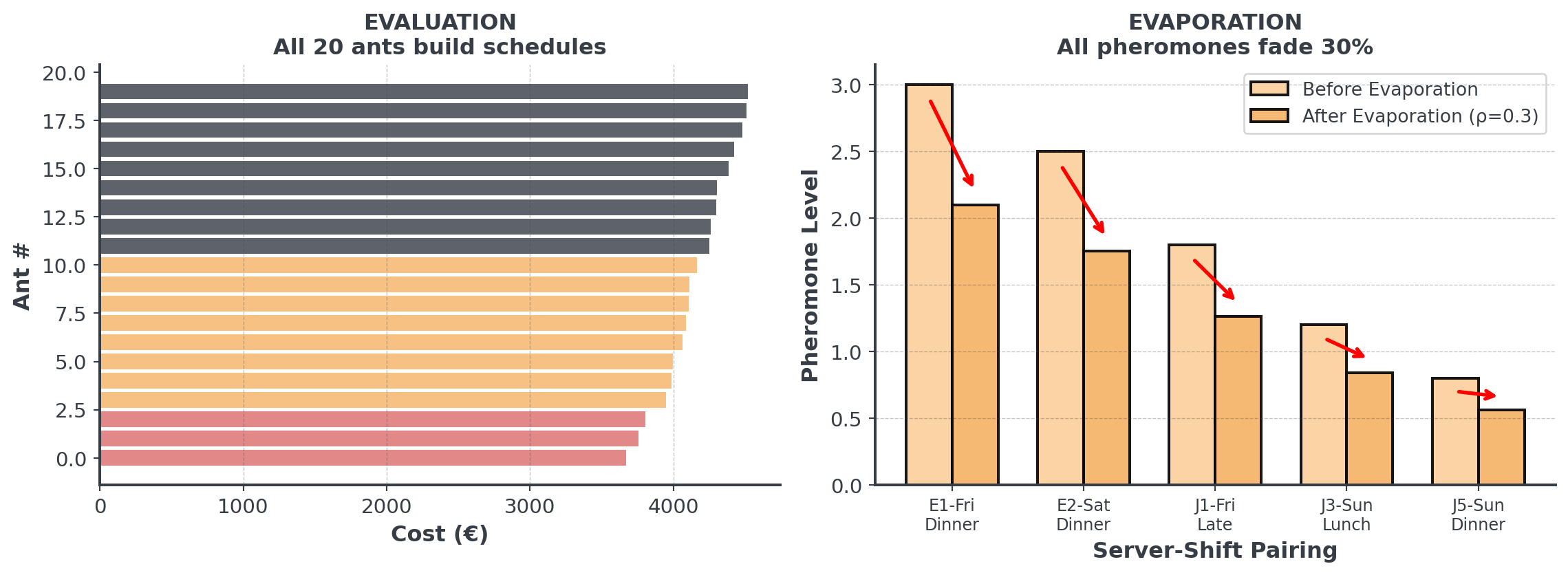
Evaporation prevents premature convergence as old patterns can fade away!

Stage 3: Reinforcement

Good ants deposit more pheromones:

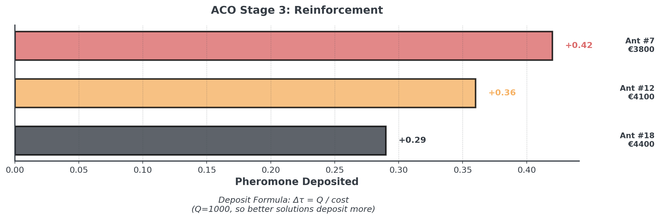
The best solutions leave the strongest trails for future iterations!

Stage 4: Evolution Over Iterations

Full ACO implementation on restaurant staffing:

. . .

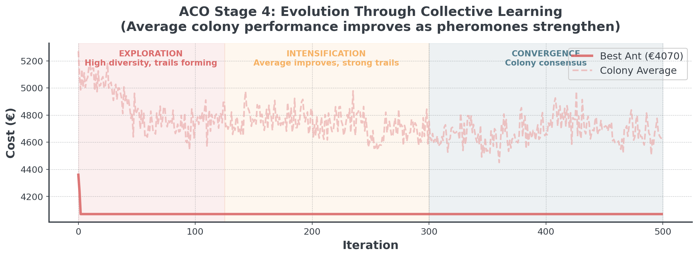
The colony learns collectively step by step.

ACO vs Other Algorithms

How does the ant colony compare?

. . .

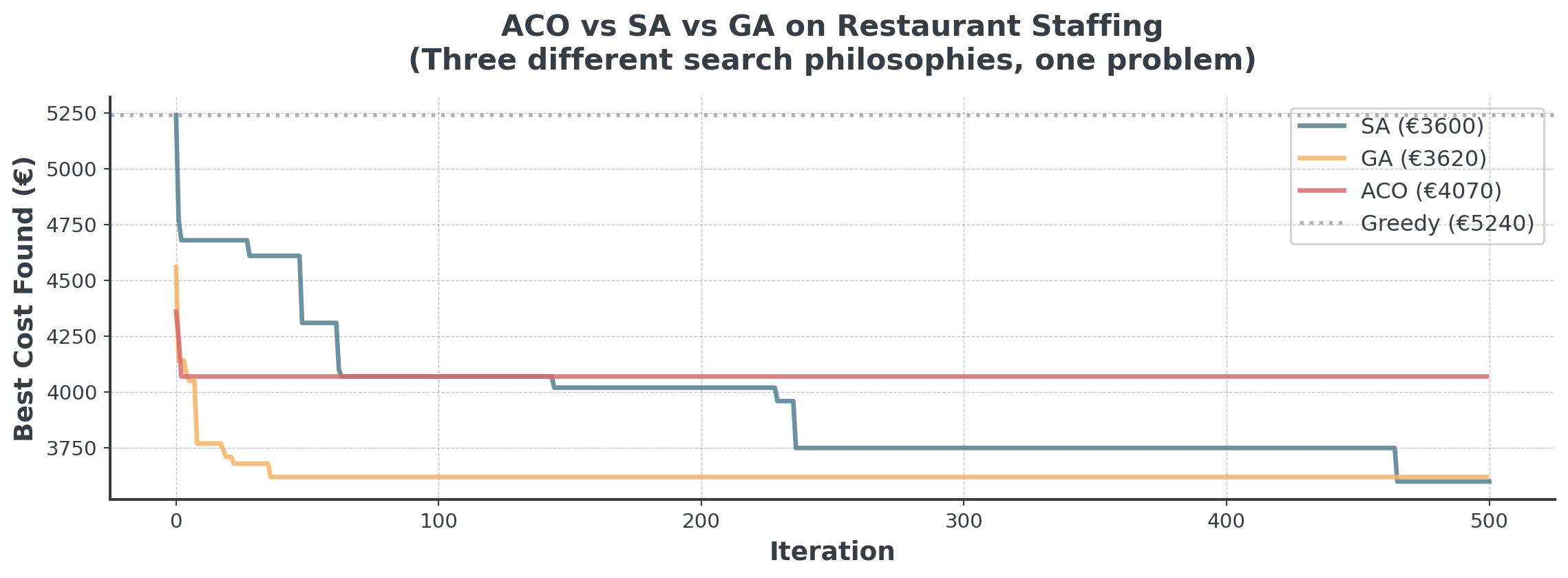
Any idea why ACO fares worse?

Why did ACO struggle?

The Right Tool for the Wrong Job

ACO is designed for Sequential Path-Finding (Graph Traversal).

Best For: “I am at City A, where should I go next?” (TSP)
Our Problem: “Who should work Friday Dinner?” (Assignment)

. . .

We forced a “Graph” algorithm onto a “Bin Packing” problem. SA and GA don’t care about geometry, so they adapted better!

Decision Framework

When to Use Which Metaheuristic?

A decision guide for algorithm selection:

Method	Time	Quality	Complexity	Best For
Random	xxxx	x	Trivial	Baseline
Greedy	xxx	xx	Simple	Quick decisions
LS	xx	xxx	Medium	Improvement
SA	xx	xxxx	Medium	Single solution
GA	x	xxxx	High	Population
TS	xx	xxx	Medium	Avoid cycles
ACO	x	xxxx	High	Changing Paths

The No Free Lunch Theorem

Why there’s no universal best algorithm:

“No Free Lunch Theorem”: No single algorithm is best for all problems. Your choice must match your problem structure:

Path/Network Problems → ACO (pheromones for paths)
Scheduling Problems → SA or Tabu (neighborhood swaps)
Complex Design → GA (population diversity)

Implementation Strategy

Guidelines for successful implementation:

Start Simple: Always try greedy first as baseline
Profile Your Problem: Understand constraints before choosing
Tune Incrementally: Don’t optimize all parameters at once
Track Progress: Monitor convergence to know when to stop
Hybrid Approaches: Combine methods (e.g., GA + Local Search)
Use AI Assistance: Bridge the “knowledge gap” with GenAI

Today’s Briefing

Today

Hour 2: This Lecture

Metaheuristics
Simulated annealing
Genetic algorithms
Tabu search & ACO

Hour 3: Notebook

Bean Counter delivery
Implement SA
Tune parameters
Compare performance

Hour 4: Competition

Restaurant staffing
Multi-objective
Schedule optimization
Justify choice!

The Competition Challenge

La Étoile Restaurant Weekend Staffing

. . .

Schedule 18 servers across 6 shifts (different lengths)
Minimize labor + experience penalties + preference costs
Ensure experienced coverage (strategic placement)
Respect 2 servers per shift requirement

. . .

Choose your metaheuristic wisely as this is a tough problem!

Parameter Tuning Strategies

How to find good parameters without wasting time:

Start with Rules of Thumb
- SA: Initial temp = max cost difference you’d accept
- GA: Population = 10-20× number of decision variables
- Tabu: Tenure (limit) = √(problem size)
Grid Search on Small Instance
- Test 3-4 values per parameter
- Use 10% of full dataset
- Example: temps = [100, 500], cooling = [0.95, 0.99]

Real-World Considerations

Technical realities when putting metaheuristics into production:

Factor	Questions to Ask
Time Budget	How long can optimization run?
Solution Quality	Need optimal or “good enough”?
Explainability	Must justify decisions?
Problem Changes	Static or dynamic data?
Team Skills	Who maintains this code?

. . .

Use the simplest method that meets your quality target. Complex metaheuristics are great but more costly to maintain!

Summary

Key Takeaways:

Metaheuristics escape local optima when exact methods fail
SA uses temperature, GA uses evolution, Tabu uses memory
Parameter tuning is critical for performance
No universal best - problem structure matters
Start simple, add complexity only if needed

Break!

Take 20 minutes, then we start the practice notebook

Next up: You’ll implement metaheuristics for Bean Counter