Management Science - From Corporate Events to Rush Hours
Introduction
Welcome to your role as Bean Counter’s Operations Manager! You’ve been tasked with solving two critical scheduling challenges that will determine the efficiency of your coffee empire:
Challenge 1: The Corporate Event (Sections 1-4)
A major tech company just ordered 20 specialty coffee drinks for their board meeting. All orders are known upfront with specific deadlines. This is a batch scheduling problem, you have complete information and need to sequence the orders optimally before starting work.
Challenge 2: The Friday Morning Rush (Sections 5-6)
Every Friday, your flagship store faces a continuous stream of orders arriving throughout the morning. You can’t see future orders and thus you must make real-time decisions. This is an online scheduling problem where orders reveal themselves over time.
These two scenarios represent fundamentally different scheduling paradigms you’ll master today!
NoteHow to Use This Tutorial
Cells marked with “YOUR CODE BELOW” expect you to write code. Test your solutions with the provided assertions. Work through sections in order as each builds on previous concepts!
import numpy as npimport pandas as pdimport matplotlib.pyplot as pltimport matplotlib.patches as mpatchesfrom datetime import datetime, timedelta# Set random seed for reproducibilitynp.random.seed(2025)print("Libraries loaded! Ready to optimize Bean Counter's operations.")
Libraries loaded! Ready to optimize Bean Counter's operations.
Section 1 - The Corporate Event Problem
The Scenario
TechCorp’s board meeting starts in 90 minutes. They’ve pre-ordered 20 specialty drinks with specific requirements. You have:
Complete information: All 20 orders known upfront
One machine: Must sequence orders optimally
Varying complexity: From simple espressos (3 min) to complex mochas (12 min)
Deadlines: Some executives need drinks early (rushed board members), others can wait (relaxed attendees)
This is static scheduling - you can plan the entire sequence before starting.
The Data Structure
Each order contains:
Order ID: Customer identifier
Processing Time: How long it takes to make
Due Time: When the customer needs it (measured from start of your shift)
Note: No arrival times! All orders are available at time 0.
# TechCorp Corporate Event - 20 pre-orders# All available at start (time 0)np.random.seed(2025)corporate_orders = []for i inrange(20): processing = np.random.choice([3, 5, 7, 10, 12], p=[0.25, 0.30, 0.25, 0.15, 0.05])# 30% tight (15-30 min), 40% medium (30-60 min), 30% relaxed (60-90 min) deadline_type = np.random.choice(['tight', 'medium', 'relaxed'], p=[0.3, 0.4, 0.3])if deadline_type =='tight': due = np.random.randint(15, 30)elif deadline_type =='medium': due = np.random.randint(30, 60)else: due = np.random.randint(60, 90) corporate_orders.append({'id': f'C{i+1:02d}', # Order-ID'processing': processing, # Time needed to process each order'due': due # Time when each order is due })df_corporate = pd.DataFrame(corporate_orders)print("TechCorp Corporate Event Orders:")print(f"Total orders: {len(corporate_orders)}")print(f"Total processing time needed: {df_corporate['processing'].sum()} minutes")print(f"Event window: 90 minutes")print(f"Tightest deadline: {df_corporate['due'].min()} minutes")print(f"Latest deadline: {df_corporate['due'].max()} minutes")print(f"\nFirst 10 orders:")print(df_corporate.head(10)[['id', 'processing', 'due']])
def calculate_metrics(schedule_df):""" Calculate key performance metrics for a schedule - Makespan: Total time to complete all orders - Avg Flow Time: Average time from start until completion - Total Tardiness: Sum of delays beyond due times - Late Orders: Count of orders completed after deadline """ metrics = {'makespan': schedule_df['completion'].max(),'avg_flow_time': schedule_df['completion'].mean(),'total_tardiness': np.maximum(0, schedule_df['completion'] - schedule_df['due']).sum(),'late_orders': (schedule_df['completion'] > schedule_df['due']).sum() }return metricsprint("Metrics function ready for comparing scheduling rules!")
Metrics function ready for comparing scheduling rules!
Exercise 1.1 - Calculate Order Slack
Slack tells you how much scheduling flexibility exists for each order. It’s the time buffer before an order becomes late.
Formula: Slack = Due Time - Processing Time
Why? If an order takes 5 minutes and is due at 20 minutes, you have 15 minutes of slack (can start anytime from 0 to 15).
NoteDataFrame Column Operations
# Create new column from calculationdf['new_col'] = df['col1'] - df['col2']# Find index of minimum valuemin_idx = df['column'].idxmin()# Get value from specific rowvalue = df.loc[min_idx, 'column_name']
# YOUR CODE BELOW# Calculate slack for each order# Add a 'slack' column to df_corporatedf_corporate['slack'] =# Calculate: due - processing# Find the most urgent order (minimum slack)# Hint: Use idxmin() to find index, then .loc[] to get the IDmost_urgent =# Find the order ID with minimum slack
Code
# Testsassert'slack'in df_corporate.columns, "Add a 'slack' column to df_corporate"assertlen(df_corporate['slack']) ==20, "Should calculate slack for all 20 orders"assert (df_corporate['slack'] == df_corporate['due'] - df_corporate['processing']).all(), \"Slack formula: due - processing"print(f"Perfect! Most urgent order: {most_urgent} with {df_corporate['slack'].min()} minutes slack")print("\nTop 5 most urgent orders:")print(df_corporate.nsmallest(5, 'slack')[['id', 'processing', 'due', 'slack']])
Section 2 - Implementing Static Scheduling Rules
Now implement three fundamental scheduling rules. For static scheduling, we:
Sort all orders by the rule’s criterion
Process them sequentially from time 0
Each order starts immediately after the previous one finishes
Rule 1: FIFO (First In, First Out)
Process orders in their original sequence (order ID order).
sorted() function sorts a list based on a criterion
lambda x: x['id'] is a mini-function that is used in sorted() saying “sort by the ‘id’ field”
def schedule_fifo_static(orders):""" Schedule orders using First In, First Out (FIFO) Process in original order """# Sort by ID to maintain original order scheduled =sorted(orders, key=lambda x: x['id'])# Calculate completion times current_time =0for order in scheduled:# In static scheduling, all orders are available at time 0# So we just start immediately after the previous order order['start'] = current_time order['completion'] = current_time + order['processing'] current_time = order['completion']return scheduled# Test FIFO# Why .copy()? We don't want to modify the original 'orders' list# Each scheduling function will modify the orders, so we give it a copyfifo_schedule = schedule_fifo_static(corporate_orders.copy())df_fifo = pd.DataFrame(fifo_schedule)print("FIFO Schedule (first 10 orders):")print(df_fifo.head(10)[['id', 'processing', 'start', 'completion', 'due']])print(f"\nTotal makespan: {df_fifo['completion'].max()} minutes")
Implement EDD to minimize tardiness by processing urgent orders first.
Structure is identical to SPT! Just change what you sort by.
# YOUR CODE BELOWdef schedule_edd_static(orders):""" Schedule orders using Earliest Due Date (EDD) Process orders with earliest deadlines first """# Sort by due date (earliest first) scheduled =# YOUR CODE# Calculate completion times current_time =0for order in scheduled: order['start'] =# YOUR CODE order['completion'] =# YOUR CODE current_time =# YOUR CODEreturn scheduled# Test your EDD implementationedd_schedule = schedule_edd_static(corporate_orders.copy())df_edd = pd.DataFrame(edd_schedule)
Code
# Testsassert df_edd.iloc[0]['due'] <= df_edd.iloc[1]['due'], "First order should have earliest due date"assert df_edd['completion'].max() == df_fifo['completion'].max(), "All schedules have same makespan"total_tardiness = np.maximum(0, df_edd['completion'] - df_edd['due']).sum()print(f"EDD implementation correct!")print(f"\nEDD Schedule (first 10 orders - sorted by due date):")print(df_edd.head(10)[['id', 'due', 'processing', 'start', 'completion']])print(f"Total tardiness: {total_tardiness:.0f} minutes")
Section 3 - Visualizing Schedules
A picture is worth a thousand schedules! Let’s create Gantt charts to visualize how each rule performs. Try to use generate AI to come up with the code to create a beautiful Gantt chart here based on the results of your schedule.
# YOUR CODE BELOW
Section 4 - Performance Comparison
Exercise 4.1 - Compare Scheduling Rules
Calculate metrics for all three rules to see which performs best.
TipCoding Hints
The calculate_metrics() function is already defined - you just call it!
It returns a dictionary with metrics like {'makespan': 29, 'avg_flow_time': 15.2, ...}
Pass the DataFrame to the function: calculate_metrics(df_fifo)
# YOUR CODE BELOW# Calculate metrics for each schedule# Hint: calculate_metrics(df_fifo) returns a dictionarymetrics_fifo =# YOUR CODEmetrics_spt =# YOUR CODEmetrics_edd =# YOUR CODE# Create comparison DataFrame# The .T transposes so methods are rowscomparison = pd.DataFrame({'FIFO': metrics_fifo,'SPT': metrics_spt,'EDD': metrics_edd}).Tprint("Performance Comparison - Corporate Event:")print(comparison.round(2))
Code
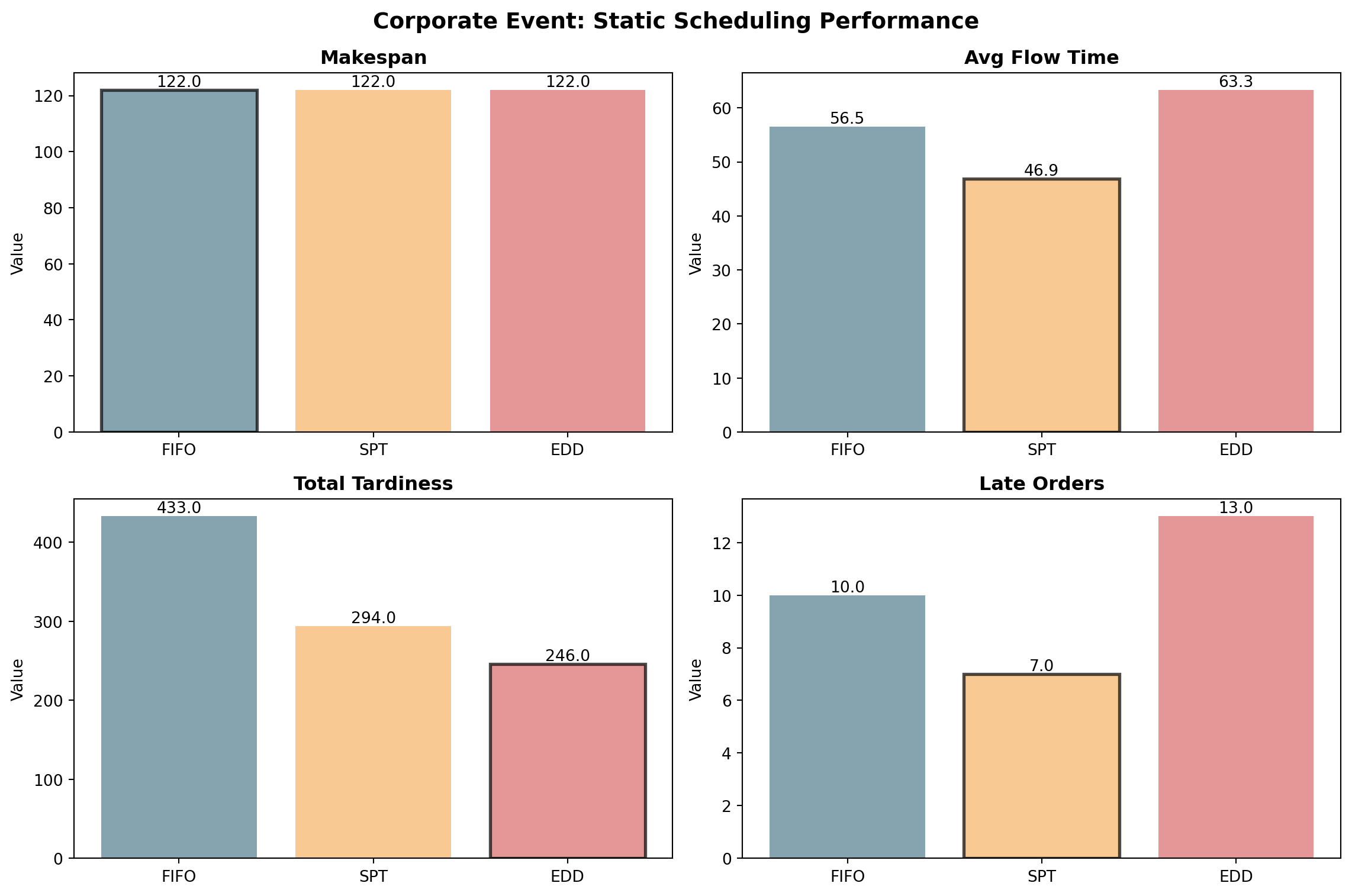
# Testsassert comparison.loc['SPT', 'avg_flow_time'] <= comparison.loc['FIFO', 'avg_flow_time'], \"SPT should have best average flow time"assert comparison.loc['EDD', 'total_tardiness'] <= comparison.loc['FIFO', 'total_tardiness'], \"EDD should minimize tardiness"assert comparison.loc['EDD', 'total_tardiness'] <= comparison.loc['SPT', 'total_tardiness'], \"EDD should beat SPT on tardiness"print("✓ Excellent analysis!")print(f"\nKey Insights:")print(f" SPT reduces avg flow time by {(1- comparison.loc['SPT', 'avg_flow_time']/comparison.loc['FIFO', 'avg_flow_time'])*100:.1f}% vs FIFO")print(f" EDD reduces tardiness by {comparison.loc['FIFO', 'total_tardiness'] - comparison.loc['EDD', 'total_tardiness']:.0f} minutes vs FIFO")print(f" EDD reduces late orders from {comparison.loc['FIFO', 'late_orders']:.0f} to {comparison.loc['EDD', 'late_orders']:.0f}")print(f" All methods have same makespan: {comparison['makespan'].iloc[0]:.0f} minutes (sum of all processing times)")
Let’s see what goes wrong if we apply static SPT to this dynamic problem:
# Apply static SPT (sorts all orders, ignores arrivals)friday_static_spt = schedule_spt_static(friday_orders.copy())df_friday_static_spt = pd.DataFrame(friday_static_spt)print("Static SPT on Friday Rush:")print(df_friday_static_spt.head(10)[['id', 'arrival', 'processing', 'start', 'completion']])print(f"\nNotice the problem: Order {df_friday_static_spt.iloc[0]['id']} starts at time 0")print(f"But it doesn't arrive until time {df_friday_static_spt.iloc[0]['arrival']:.1f}!")print(f"This creates {df_friday_static_spt.iloc[0]['arrival']:.1f} minutes of idle time.")
Static SPT on Friday Rush:
    id  arrival  processing  start  completion
0  F04      5.6           1      0           1
1  F10     13.4           1      1           2
2  F13     23.6           1      2           3
3  F23     46.9           1      3           4
4  F25     48.0           1      4           5
5  F01      0.0           2      5           7
6  F03      2.4           2      7           9
7  F05      5.8           2      9          11
8  F06      6.5           2     11          13
9  F08      9.1           2     13          15

Notice the problem: Order F04 starts at time 0
But it doesn't arrive until time 5.6!
This creates 5.6 minutes of idle time.
Static scheduling on online problems creates idle time!
Static SPT sorts all orders by processing time, then tries to do the shortest first. But if that order hasn’t arrived yet, the machine sits idle waiting.
We need dynamic dispatching that only considers orders that have already arrived.
Section 6 - Dynamic Dispatching
The Dynamic Dispatching Algorithm
Instead of sorting everything upfront, we make decisions one at a time as the machine becomes free:
Start with current_time = 0
While there are unscheduled orders:
Find which orders have arrival <= current_time (the “available pool”)
If no orders available, jump forward to the next arrival
Apply your rule (FIFO/SPT/EDD) to choose from the available pool
Schedule that order, update time, repeat
This simulates real-time decision-making!
Exercise 6.1 - Implement Dynamic SPT
Implement SPT with dynamic dispatching for Bean Counter.
TipDynamic Scheduling Logic
Key difference from static: You can only schedule orders that have already arrived!
Use a while remaining: loop (not a for loop over pre-sorted list)
Filter to available = [orders where arrival <= current_time]
If no available orders, jump forward: current_time = min(arrival of remaining)
Then apply SPT to the available pool
NoteList Comprehension for Filtering
List comprehension creates a new list based on a condition:
# General patternnew_list = [item for item in old_list if condition]# Example: filter numbers > 5numbers = [3, 7, 2, 9, 1, 6]big_numbers = [n for n in numbers if n >5]# Result: [7, 9, 6]# Filter orders by arrival timeavailable = [order for order in remaining if order['arrival'] <= current_time]
# YOUR CODE BELOWdef schedule_spt_dynamic(orders):""" Schedule orders using DYNAMIC Shortest Processing Time At each decision point, choose shortest job among those that have arrived """ scheduled = [] remaining = [o.copy() for o in orders] # Make copies to avoid modifying originals current_time =0while remaining:# Find available orders (already arrived)# Use list comprehension: [o for o in remaining if ...] available =# YOUR CODE: list of orders where arrival <= current_time# If nothing available, jump to next arrivalifnot available:# Find earliest arrival among remaining orders current_time =# YOUR CODE: min arrival time of remaining orders# Now re-filter for available orders available =# YOUR CODE: update available orders# Choose shortest processing time among available# Use min() with key=lambda next_order =# YOUR CODE: min(available, key=lambda ...)# Schedule it next_order['start'] = current_time next_order['completion'] = current_time + next_order['processing'] current_time = next_order['completion']# Move from remaining to scheduled scheduled.append(next_order) remaining.remove(next_order)return scheduled# Test dynamic SPTfriday_dynamic_spt = schedule_spt_dynamic(friday_orders)df_friday_dynamic_spt = pd.DataFrame(friday_dynamic_spt)
Code
# Testsassertall(df_friday_dynamic_spt['start'] >= df_friday_dynamic_spt['arrival']), \"All orders should start at or after their arrival time"# Calculate idle time for both approachesstatic_idle =sum(max(0, row['arrival'] - (df_friday_static_spt.iloc[i-1]['completion'] if i >0else0))for i, row in df_friday_static_spt.iterrows())dynamic_idle =sum(max(0, row['start'] - (df_friday_dynamic_spt.iloc[i-1]['completion'] if i >0else0))for i, row in df_friday_dynamic_spt.iterrows())print("Excellent! Dynamic SPT implementation is correct!")print(f"\nDynamic vs Static SPT on Friday Rush:")print(f" • Static makespan (with arrival violations!): {df_friday_static_spt['completion'].max():.1f} minutes")print(f" • Dynamic makespan (no violations): {df_friday_dynamic_spt['completion'].max():.1f} minutes")print(f" • Change: {df_friday_static_spt['completion'].max() - df_friday_dynamic_spt['completion'].max():.1f} minutes faster")print(f" • Dynamic idle time: {dynamic_idle:.1f} minutes")
Exercise 6.2 - Implement Dynamic EDD
Now implement EDD with dynamic dispatching to minimize tardiness in the Friday rush.
# YOUR CODE BELOWdef schedule_edd_dynamic(orders):""" Schedule orders using DYNAMIC Earliest Due Date At each decision point, choose order with earliest deadline among available orders """ scheduled = [] remaining = [o.copy() for o in orders] current_time =0while remaining:# YOUR CODE: Find available orders available =# [orders where arrival <= current_time]# YOUR CODE: Handle no available ordersifnot available: current_time =# min arrival of remaining available =# update available# YOUR CODE: Choose earliest due date next_order =# Hint: Just change the key from SPT# Schedule it (same as SPT) next_order['start'] = current_time next_order['completion'] = current_time + next_order['processing'] current_time = next_order['completion'] scheduled.append(next_order) remaining.remove(next_order)return scheduled# Test dynamic EDDfriday_dynamic_edd = schedule_edd_dynamic(friday_orders)df_friday_dynamic_edd = pd.DataFrame(friday_dynamic_edd)
Code
# Testsassertall(df_friday_dynamic_edd['start'] >= df_friday_dynamic_edd['arrival']), \"All orders should start at or after arrival"metrics_dynamic_spt = calculate_metrics(df_friday_dynamic_spt)metrics_dynamic_edd = calculate_metrics(df_friday_dynamic_edd)assert metrics_dynamic_edd['total_tardiness'] <= metrics_dynamic_spt['total_tardiness'], \"EDD should minimize tardiness better than SPT"print("✓ Dynamic EDD implementation correct!")print(f"\nFriday Rush: Dynamic SPT vs Dynamic EDD")print(f" • SPT avg flow time: {metrics_dynamic_spt['avg_flow_time']:.1f} minutes")print(f" • EDD avg flow time: {metrics_dynamic_edd['avg_flow_time']:.1f} minutes")print(f" • SPT total tardiness: {metrics_dynamic_spt['total_tardiness']:.1f} minutes")print(f" • EDD total tardiness: {metrics_dynamic_edd['total_tardiness']:.1f} minutes")print(f" • SPT late orders: {metrics_dynamic_spt['late_orders']:.0f}")print(f" • EDD late orders: {metrics_dynamic_edd['late_orders']:.0f}")
You’ve now mastered both static and dynamic scheduling approaches! In the next notebook, you’ll tackle the Bike Factory Competition where you’ll apply these scheduling techniques to a real two-stage manufacturing problem.
In the following lectures, you’ll then learn advanced techniques like local search and metaheuristics that can improve even the best greedy solutions by intelligently exploring schedule variations.
Your Bean Counter operations are now optimized for both planning and real-time scenarios!