Dealing with Uncertainty

Lecture 4 - Management Science

Author

Dr. Tobias Vlćek

Introduction

Client Briefing: TechVenture Innovation Fund

. . .

CEO’s Dilemma:

“We have €2M to invest in 2 of 4 startups. Each promises great returns, but the future is uncertain. How do we make the best choice without just gambling?”

Business: Valuing Uncertainty

Question: Why can’t we just pick the two startups with the highest average returns?

. . .

  • Hidden Risk: A startup with 30% average return but 50% chance of failure might be worse than 20% return with 5% failure chance
  • Portfolio Effects: Two risky startups together might amplify risk beyond acceptable levels
  • Tail Events: The worst-case scenario can matter as much as the average case

. . .

Common Pitfall: Optimizing on averages ignores the distribution of outcomes.

Real-World Examples

Where uncertainty modeling is critical:

Netflix Series Decisions

  • Will a show hit 10M viewers?
  • Range: 500K to 50M
  • Investment: €20M per season

Pharmaceutical R&D

  • Will the drug pass trials?
  • Success rate: 10-20%
  • Investment: €1B over 10 years

. . .

When decisions are expensive and outcomes are uncertain, Monte Carlo simulation can be helpful to reduce risk and maximize value!

Core Concepts

Rolling the Dice 10,000 Times I

Question: If you roll two dice, what’s the probability of getting exactly 7 as result?

. . .

Method 1: Math

  • Count combinations: (1,6), (2,5), (3,4), (4,3), (5,2), (6,1)
  • Total combinations: 36
  • Probability: 6/36 = 16.67%

Rolling the Dice 10,000 Times II

Question: If you roll two dice, what’s the probability of getting exactly 7 as result?

. . .

Method 2: Simulation

import numpy as np
np.random.seed(42)

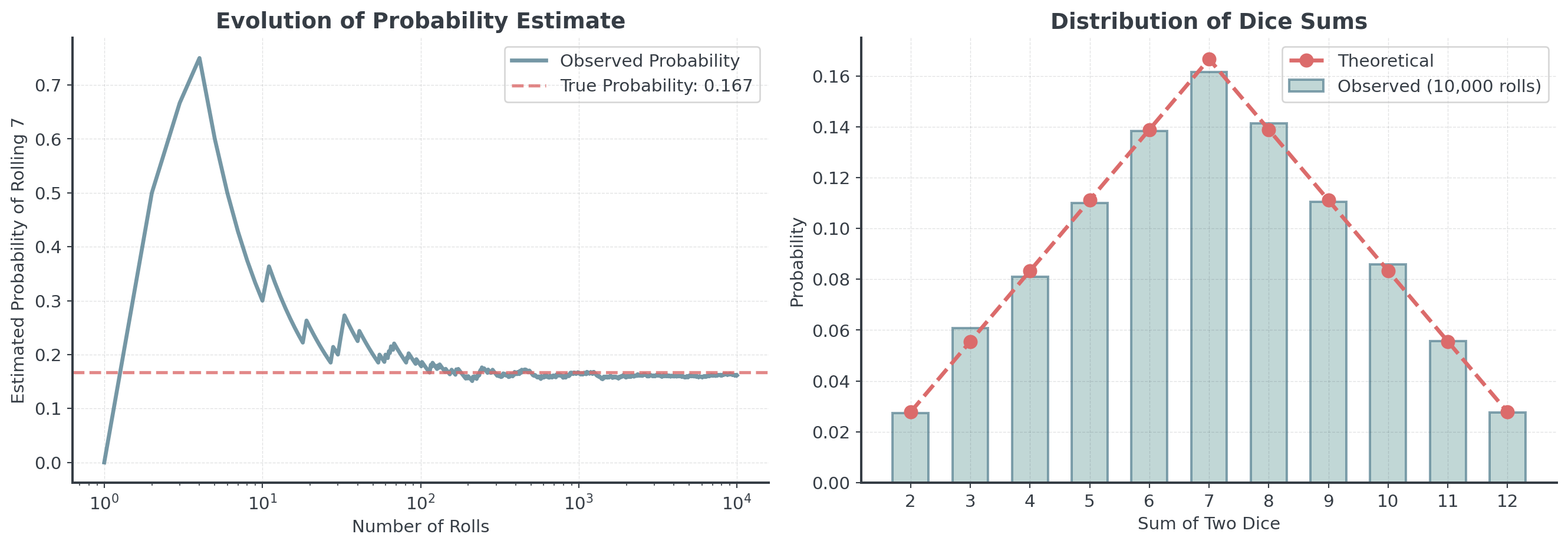
# Roll two dice 10,000 times
dice1 = np.random.randint(1, 7, size=10_000)
dice2 = np.random.randint(1, 7, size=10_000)
total = dice1 + dice2

# What fraction equals 7?
probability = (total == 7).mean()
print(f"Simulated probability of rolling 7: {probability:.1%}")
Simulated probability of rolling 7: 16.2%

How Probability Converges

. . .

As we roll more dice, the estimated probability converges to the true value (16.7%)

The Law of Large Numbers

Fundamental Principle: As sample size increases, sample average converges to the true expected value

. . .

If \(X_1, X_2, \ldots, X_n\) are independent random samples from the same distribution with mean \(\mu\):

\[\text{As } n \to \infty, \quad \bar{X}_n = \frac{1}{n}\sum_{i=1}^n X_i \to \mu\]

. . .

This is WHY simulations works. More simulations = better estimates!

The Central Limit Theorem

Another Fundamental Principle: The sum of many random variables tends toward a normal distribution

. . .

What it means:

  • Even if individual returns are NOT normally distributed…
  • The portfolio of many assets WILL be approximately normal
  • The average of many simulations WILL be approximately normal

. . .

For Business: This is why we can use normal distributions to model portfolio returns, even when individual assets have skewed or unusual distributions!

Why This Matters for Business

Question: How many simulations do we need for reliable results?

. . .

# Test convergence with different sample sizes
sample_sizes = [10, 100, 1000, 10000, 100000]
estimates = []

for n in sample_sizes:
    dice1 = np.random.randint(1, 7, size=n)
    dice2 = np.random.randint(1, 7, size=n)
    total = dice1 + dice2
    prob = (total == 7).mean()
    estimates.append(prob)
    print(f"n={n:6d}: Estimated probability = {prob:.4f}")
n=    10: Estimated probability = 0.2000
n=   100: Estimated probability = 0.1900
n=  1000: Estimated probability = 0.1480
n= 10000: Estimated probability = 0.1652
n=100000: Estimated probability = 0.1670

Practical Guidelines

How many simulations should you run?

  • Quick exploration: 10,000 simulations
    • Good for initial insights, prototyping
  • Critical decisions: 100,000+ simulations
    • Financial risk models, regulatory compliance
  • When to stop: When more simulations don’t change conclusion

. . .

If your decision changes with 10x more simulations, you didn’t run enough!

Monte Carlo Method

The Monte Carlo Method

Three Simple Steps:

  1. Model the Uncertainty:
    • Define probability distributions for unknown variables
  2. Simulate Many Scenarios:
    • Generate thousands of possible outcomes
  3. Analyze the Results:
    • Calculate statistics from the simulation

. . .

Monte Carlo Casino in Monaco inspired the method’s development in the 1940s.

Step 1: Model the Uncertainty

Key Function: np.random.normal(loc, scale, size)

  • loc: The center (mean/average)
  • scale: The spread (standard deviation)
  • size: How many samples to generate

. . .

# AI-Growth: average 38% return, ±25% volatility
returns = np.random.normal(loc=0.38, scale=0.25, size=10_000)
print(f"Mean return: {returns.mean():.1%}")
print(f"Std deviation: {returns.std():.1%}")
print(f"Minimum: {returns.min():.1%}")
print(f"Maximum: {returns.max():.1%}")
Mean return: 38.8%
Std deviation: 24.8%
Minimum: -67.0%
Maximum: 125.7%

Expected Returns

Let’s calculate percentiles with np.percentile().

. . .

Question: Do you still know what a percentile is?

. . .

print(f"\nPercentiles:")
print(f"  5th: {np.percentile(returns, 5):.1%} (worst 5% of scenarios)")
print(f" 25th: {np.percentile(returns, 25):.1%} (worst 25% of scenarios)")
print(f" 50th: {np.percentile(returns, 50):.1%} (median)")
print(f" 75th: {np.percentile(returns, 75):.1%} (best 25% of scenarios)")
print(f" 95th: {np.percentile(returns, 95):.1%} (best 5% of scenarios)")

Percentiles:
  5th: -2.7% (worst 5% of scenarios)
 25th: 22.1% (worst 25% of scenarios)
 50th: 38.9% (median)
 75th: 55.7% (best 25% of scenarios)
 95th: 78.6% (best 5% of scenarios)

Understanding the Distribution

Question: Before we plot, what shape do you expect for np.random.normal()?

. . .

Risk Analysis

Question: What’s the probability that AI-Growth loses money?

. . .

# Calculate risk metrics
prob_loss = (returns < 0).mean() # proportion of returns that are less than zero
prob_double = (returns > 1.0).mean()  # proportion greater than 100%

print(f"Probability of loss: {prob_loss:.1%}")
print(f"Probability of doubling money: {prob_double:.1%}")
Probability of loss: 6.0%
Probability of doubling money: 0.8%

. . .

With 6 % chance of loss, AI-Growth is relatively safe. Easy for one startup, right?

Different Distributions

Attention: Not everything follows a normal distribution!

Overview

# Most common in nature/business
# Bell-shaped, symmetric
returns = np.random.normal(mean, std, size)

# Example: CloudAI startup returns
cloudai = np.random.normal(0.25, 0.15, 10000)  # 25% ± 15%

Main Characteristics:

  • Symmetric bell curve
  • Most values cluster around mean
  • Common in nature and business
# Equal probability across range
# Example: FinFlow returns between 10-35%
returns = np.random.uniform(0.10, 0.35, size)

# Example: FinFlow startup returns
finflow = np.random.uniform(0.10, 0.35, 10000)  # 10-35% equally likely

Main Characteristics:

  • All values equally likely
  • Hard boundaries (min/max)
  • Good for modeling complete uncertainty within range
# Time between events
# Example: Customer arrivals, equipment failure
times = np.random.exponential(scale, size)

# Example: Time between customer arrivals (minutes)
arrivals = np.random.exponential(5, 10000)  # Average 5 minutes

Main Characteristics:

  • Many small values, few large ones
  • Always positive
  • Common for waiting times and rare events

Portfolios

Combining Investments

Suppose we have the following startups:

CloudAI, GreenGrid, HealthTrack, FinFlow

. . .

Question: If we must pick 2 of 4, how many unique pairs exist?

. . .

The Math:

\[\binom{4}{2} = \frac{4!}{2! \times 2!} = \frac{4 \times 3 \times 2 \times 1}{(2 \times 1) \times (2 \times 1)} = \frac{24}{4} = 6\]

. . .

Each combination has different risk-return characteristics!

Four Startup Profiles

. . .

Question: Which startup is the best choice?

Key Metrics for Decision Making

Question: Which metrics matter most for investment decisions?

  • Expected Return: Average outcome across all scenarios
  • Volatility (Risk): Standard deviation of returns
  • Probability of Loss: How often do we lose money?
  • Upside Potential: Chance of exceptional returns (>50%)
  • Tail Risk: What happens in the worst 10% of cases?

. . .

No metric tells the whole story. Investors consider multiple dimensions of risk and return.

Understanding Tail Risk

Tail Risk: The danger lurking in worst-case scenarios

Expected Shortfall (ES)

  • Average loss in worst X% of cases
  • Goes beyond simple probability
  • Measures depth of potential losses
  • Critical for risk management

. . .

A portfolio with higher average returns might have catastrophic tail risk. Always look at the extremes!

Correlation & Dependence

The Independence Assumption

So far, we’ve assumed startups succeed or fail independently.

. . .

Independent Events:

  • CloudAI’s success doesn’t affect GreenGrid’s success
  • Each startup faces separate, unrelated risks
  • Portfolio risk = Average of individual risks

. . .

Question: Is this realistic in the real world?

. . .

Reality Check: Many business risks are correlated! Economic downturns, market trends, and technology shifts affect multiple companies simultaneously.

What is Correlation?

Correlation measures how two variables move together.

\[\rho_{X,Y} = \frac{\text{Cov}(X,Y)}{\sigma_X \sigma_Y} \quad \text{where } -1 \leq \rho \leq 1\]

. . .

Interpreting Correlation:

  • ρ = +1: Perfect positive correlation (move together)
  • ρ = 0: No correlation (independent)
  • ρ = -1: Perfect negative correlation (move opposite)

Correlation in Practice

. . .

In Python: np.corrcoef(returns1, returns2) calculates correlation

Why Correlation Matters

Two AI startups in your portfolio:

Scenario 1: Independent (ρ = 0)

  • One fails due to technical issues, other succeeds
  • Risk is averaged out

Scenario 2: Positively Correlated (ρ = 0.8)

  • Both rely on same AI infrastructure provider - risk is amplified!

. . .

Diversification only reduces risk when investments are not highly correlated!

Impact on Portfolio Risk

. . .

Higher correlation = Wider distribution = More risk!

Real-World Correlation Examples

Common sources of correlation in business:

  • Industry-specific: All tech startups affected by downturn
  • Geographic: All European companies affected by EU regulations
  • Supply chain: Multiple companies relying on same supplier
  • Macroeconomic: Interest rates, inflation affect most businesses

. . .

Diversification: Choose investments with LOW correlation to reduce portfolio risk!

When Diversification Fails

. . .

2008 Financial Crisis: Many “diversified” portfolios collapsed due to correlations!

When Monte Carlo?

When to Use Monte Carlo

Question: For our simple startup examples so far, do we really NEED Monte Carlo?

. . .

Short answer: No! For basic mean/variance calculations, we can use analytical formulas.

. . .

So when is Monte Carlo truly necessary?

Necessary vs. Convenient

You can use math (analytical solutions):

  • Simple distributions: Mean and variance of normal distributions
  • Linear combinations: Portfolio of independent assets

. . .

You NEED Monte Carlo when:

  • Complex dependencies: Nonlinear relationships
  • Path-dependent problems: Outcome depends on a sequence
  • No closed-form solution: The math is intractable

Real Monte Carlo Applications

Where Monte Carlo is ESSENTIAL, not just convenient:

1. Option Pricing with Path Dependencies

# Payoff depends on AVERAGE price over time
n_simulations = 10000; strike_price = 105; payoffs = []
for sim in range(n_simulations):
    prices = [100]  # Starting price
    for day in range(365):
        prices.append(prices[-1] * (1 + np.random.normal(0.001, 0.02)))
    payoff = max(0, np.mean(prices) - strike_price)
    payoffs.append(payoff)
payoffs = np.array(payoffs)
print(f"Average option value: ${payoffs.mean():.2f}")
print(f"Probability of profit: {(payoffs > 0).mean():.1%}")
Average option value: $19.58
Probability of profit: 68.9%

Real Monte Carlo Applications II

Real Monte Carlo Applications III

2. Supply Chain with Cascading Effects

# Each stage affects the next (nonlinear dependencies)
n_simulations = 10000; factory_capacity = 150; demand = 120; price = 5
penalty = 10; revenues = []

for sim in range(n_simulations):
    parts_delivered = np.random.poisson(100)
    production = min(parts_delivered, factory_capacity)
    if production >= demand:
        revenue = demand * price
    else:
        revenue = production * price - penalty
    revenues.append(revenue)

revenues = np.array(revenues)
print(f"Average revenue: ${revenues.mean():.2f}")
print(f"Worst-case revenue: ${revenues.min():.2f}")
Average revenue: $489.22
Worst-case revenue: $325.00

Real Monte Carlo Applications IV

Real Monte Carlo Applications V

3. Project Management with Sequential Risks

# Project phases must happen in order, later phases only if earlier succeed
n_simulations = 10000; shape = 2; scale = 10; project_times = []

for sim in range(n_simulations):
    total_time = 0
    for phase in ['design', 'build', 'test', 'deploy']:
        # Each phase has uncertain duration
        phase_time = np.random.gamma(shape, scale)
        total_time += phase_time
        if np.random.random() < 0.1:
            total_time += phase_time * 0.5  # Rework time
    project_times.append(total_time)

project_times = np.array(project_times)
print(f"Average project duration: {project_times.mean():.1f} days")
print(f"90th percentile: {np.percentile(project_times, 90):.1f} days")
Average project duration: 84.3 days
90th percentile: 125.2 days

Real Monte Carlo Applications VI

Example: Why Still Useful?

Question: If we can calculate variance analytically, why simulate?

. . .

  • Visualization: Seeing the full distribution is intuitive
  • Flexibility: When problems become complex, simulation adapts
  • Extensions: Practice for complex problem

. . .

Think of our examples as learning the tool on simple problems so you can solve complex ones where Monte Carlo is required!

When NOT to Use Monte Carlo

Even when you CAN use Monte Carlo, sometimes you shouldn’t:

. . .

  • Simple analytical solution exists and suffices
    • Use math directly: faster, more precise, easier to understand
  • Can’t reasonably estimate input distributions
    • Garbage in = garbage out; need solid basis for assumptions
  • Problem is deterministic (no uncertainty)
    • Simulation adds complexity without value

. . .

Simulation is a tool for managing uncertainty, not creating false precision!

Making Smart Decisions

Decision Framework

  1. Define Your Risk Tolerance
    • Can you afford to lose money and what’s your time horizon?
    • Are you risk-averse or risk-seeking?
  2. Evaluate Multiple Metrics
    • Don’t just maximize returns, consider volatility and risk
    • Look at probability of achieving goals
  3. Scenario Test
    • What if distributions change or a company fails?

The Plan for the Day

Hour 1:

Lecture

  • Concepts
  • Examples
  • Visualization

Hour 2:

Practice Notebook

  • Simulation
  • Hands-on coding
  • Build your skills

Hours 3-4:

Competition

  • TechVenture
  • Team collaboration
  • €2M investment

. . .

Remember: The lecture gives you concepts. The notebook gives you practice. The competition tests your skills!

Hour 2: Simulation

Your Practice Case: Bean Counter Expansion

  • Model uncertain variables (customers, spending)
  • Combine multiple uncertainties
  • Calculate business metrics (VaR, profit probability)
  • Make data-driven recommendations

Hours 3-4: The Challenge

TechVenture Investment Competition

  • Your Budget: €2 million
  • Your Choice: Pick 2 of 4 startups
  • Your Goal: Maximize risk-adjusted returns
  • Your Deliverable: One-slide recommendation + 3-minute pitch

. . .

Consider multiple risk metrics and prepare a clear justification!

. . .

Prizes: 10 / 6 / 3 bonus points for top three teams!

Key Takeaways

What You’ve Learned Today

Concepts

  • Monte Carlo simulation
  • Probability distributions
  • Risk has multiple dimensions
  • Expected Value vs. Variance
  • Correlation and dependence

Skills

  • Using np.random for simulation
  • Calculating risk metrics
  • Visualizing uncertainty
  • Comparing portfolios
  • Understanding correlation

. . .

Monte Carlo doesn’t predict THE future - it shows possible futures! And correlation can amplify or reduce risk!

Next Week

Forecasting the Future

  • Moving from simulation to prediction
  • Time series analysis
  • Trend and seasonality detection
  • Measuring forecast accuracy

. . .

Now, short break and then we start coding!