Better Routing

Lecture 7 - Management Science

Author

Dr. Tobias Vlćek

Introduction

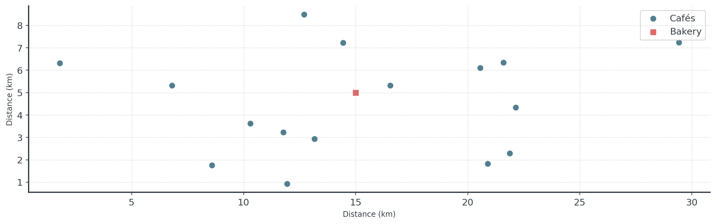
Client Briefing: Artisan Bakery

. . .

Master Baker’s Morning Dilemma:

“Every morning at 5:00, our delivery van leaves with fresh bread for 16 cafés across the city. Our driver currently takes much too long using his ‘intuition’ for the route. The fuel costs are killing us, and worse, some cafés get their bread late.”

The Delivery Challenge

Artisan Bakery’s daily logistics puzzle:

16 Cafés: Each expecting fresh bread by 8:00
One Van: Unlimited capacity, must visit all locations
Time Windows: 3 cafés open early (6:30) and need priority
Current Problem: Driver uses “gut feeling” for routing

. . .

The Stakes: Poor routing costs plus reputation damage from late deliveries!

Quick Recap: Greedy Decisions

Last week we learned greedy algorithms for scheduling:

SPT: Process shortest jobs first
EDD: Process by earliest due date
Fast & Simple: Made quick decisions, no looking back

. . .

Question: Can we use the same greedy approach for routing?

. . .

Today: We’ll start greedy, then learn how to improve solutions with local search!

The Routing Problem

The Traveling Salesman Problem

Visit all locations exactly once, minimize total distance.

. . .

Compute Everything?

How many unique tours exist? With depot, n!/2 unique tours.

. . .

If your computer checks 1 million routes per second:

4 cafés: 4!/2 = 12 tours → 0.000012 seconds ✓
8 cafés: 8!/2 = 20,160 tours → 0.02 seconds ✓
12 cafés: 12!/2 = 239,500,800 tours → 4 minutes ~
16 cafés: 16!/2 = 10,461,394,944,000 tours → 4 months! ✗
20 cafés: 20!/2 → 38,573 years! ✗

. . .

The Reality: Exact approach would take longer than the universe has existed!

The “Cost” of Complexity

Why buying a faster computer won’t help:

P: Tasks that can be solved in polynomial time
- Like sorting a spreadsheet or calculating payroll
- These are safe, predictable, and easy to automate
NP: Easy to check, hard to solve
- Analogy: easy to check if a specific password works
- Very hard to guess a password by trying every combination!

. . .

TSP optimization where we find minimum cost tour → NP-Hard. This means no known algorithm can find the perfect solution quickly for large problems.

Graph Theory Foundations

What is a Graph?

A graph \(G = (V, E)\) consists of:

Vertices (V): The nodes or points (bakery + cafés)
Edges (E): The connections between vertices (roads)
Weight Function: \(w\) assigns costs to edges (distances)

. . .

For our bakery problem:

\(|V| = 17\) (1 bakery + 17 cafés)
\(|E| = \binom{17}{2} = 136\) possible connections
Each edge \((i,j)\) has weight \(w_{ij}\) = distance between \(i\) and \(j\)

Complete vs. Sparse Graphs

Different graph structures lead to different complexities:

Complete Graph: All vertices connected to each other
- TSP: \((n-1)!/2\) unique tours
- Real roads: Usually complete (drive between any two points)
Sparse Graph: Limited connections between vertices
- Fewer edges = fewer possible routes
- Examples: Public transit networks, restricted road access

. . .

Density dramatically affects both problem difficulty and solution approaches!

Hamiltonian Cycles and Tours

Mathematical foundation of the TSP:

Hamiltonian Path: Visits each vertex exactly once
Hamiltonian Cycle: Hamiltonian path that returns to start vertex
TSP Tour: Minimum weight Hamiltonian cycle

. . .

Mathematical Definition: A tour \(T = (v_1, v_2, ..., v_n, v_1)\) where:

Each \(v_i \in V\) appears exactly once (except start/end)
Total weight: \(w(T) = \sum_{i=1}^{n} w_{v_i, v_{i+1}}\) (where \(v_{n+1} = v_1\))

. . .

Goal: Find tour \(T^*\) such that \(w(T^*) = \min_{T \in \mathcal{H}} w(T)\)

Distance Functions and Metrics

The weight function can have different properties:

Identity: \(d(i,i) = 0\) \(i \in V\)
Symmetry: \(d(i,j) = d(j,i)\) \(i,j \in V\)
Triangle Inequality: \(d(i,k) \leq d(i,j) + d(j,k) \quad \forall i,j,k \in V\)

. . .

Common Distance Functions:

Euclidean: \(d(i,j) = \sqrt{(x_i - x_j)^2 + (y_i - y_j)^2}\)
Manhattan: \(d(i,j) = |x_i - x_j| + |y_i - y_j|\)
Real road distances: Often violate triangle inequality!

Greedy Construction

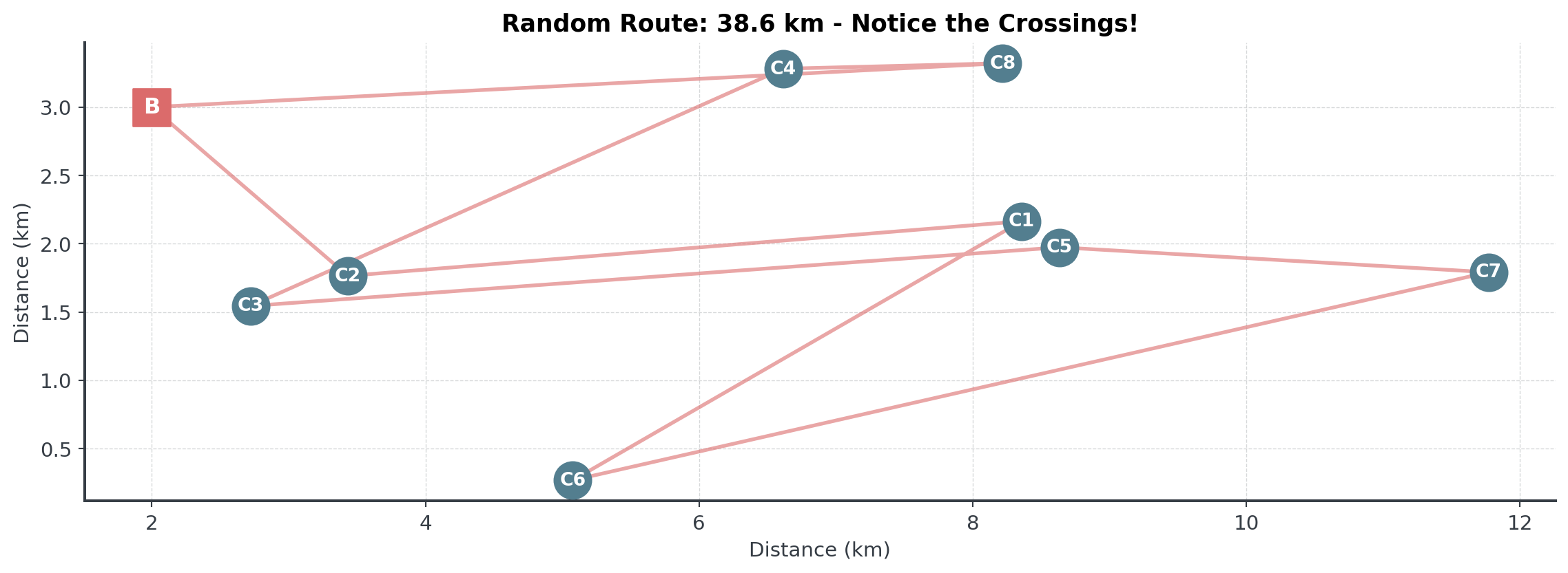
A Bad Start: Random Route

What happens if we pick cafés randomly?

. . .

. . .

Random selection creates routes with many crossings and inefficiencies.

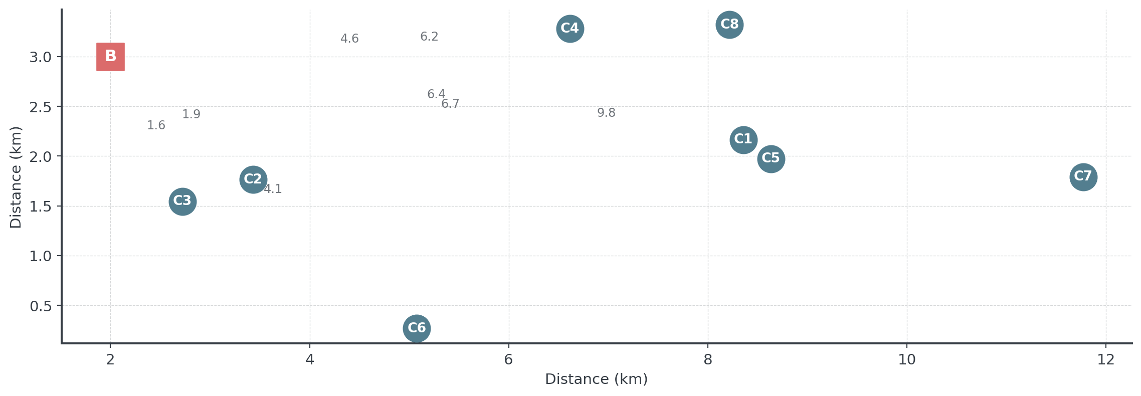
Nearest Neighbor: The Problem

Given these 8 cafés, which should we visit first?

. . .

Question: Using nearest neighbor, which café would you visit first?

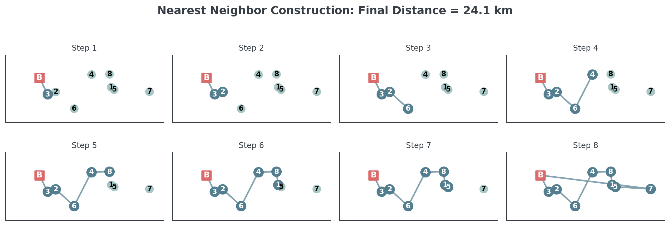
Nearest Neighbor: The Algorithm

Build a route by always visiting the closest unvisited location.

Start at the bakery
Find the nearest unvisited café
Go there
Repeat until all visited
Return to bakery

. . .

Intuition: Like picking low-hanging fruit - grab what’s easiest (nearest) first!

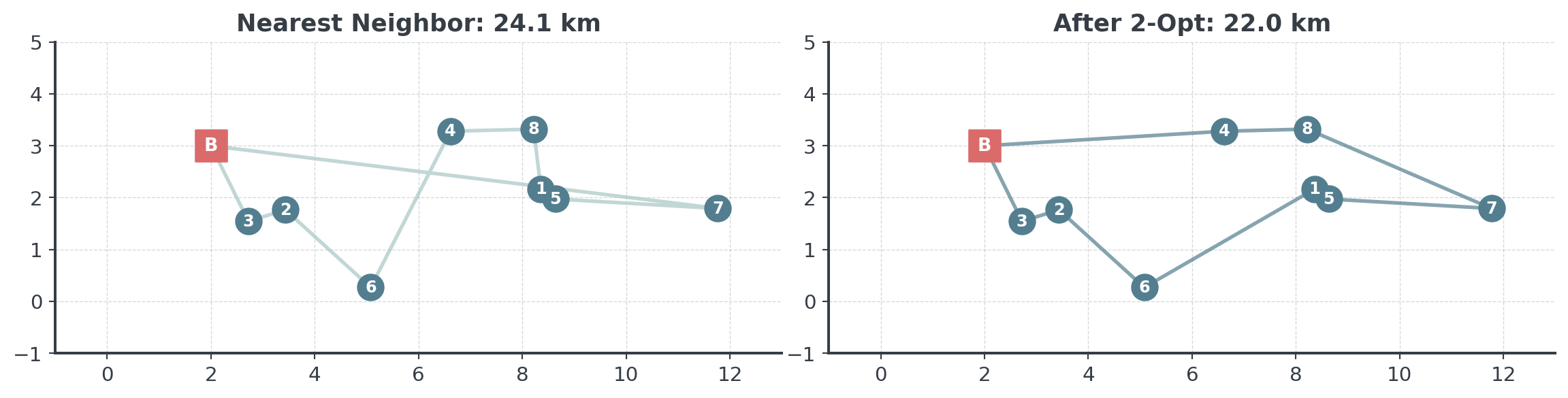
Nearest Neighbor: The Solution

Let’s see how nearest neighbor builds the route step by step:

. . .

Farthest insertion builds a more balanced tour by establishing the outer structure first!

Farthest Insertion: The Problem

Same 8 cafés - but now we’ll use a different strategy:

. . .

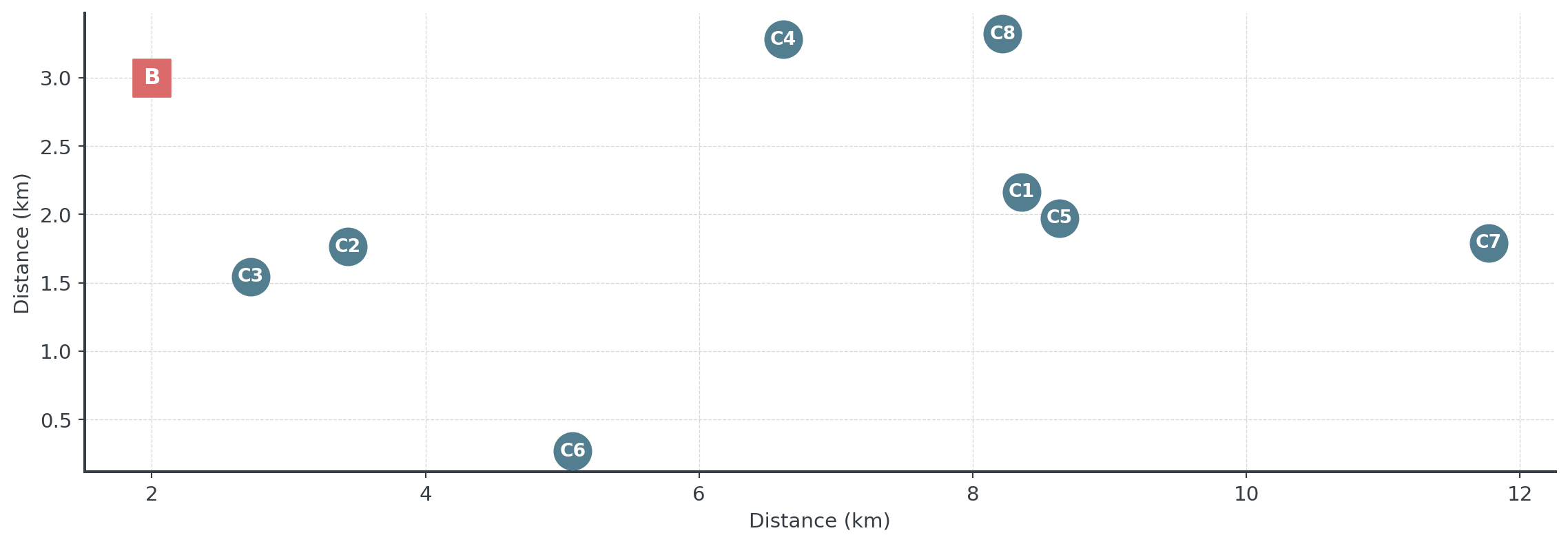
The farthest point is our start!

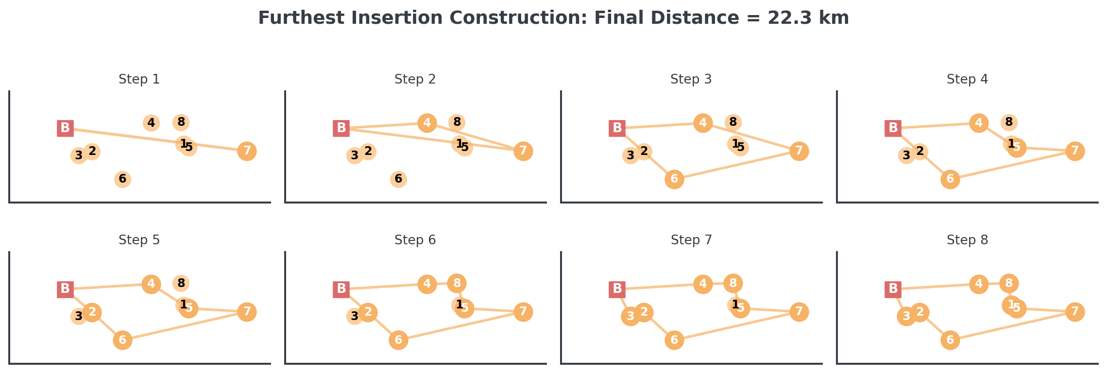
Farthest Insertion: The Algorithm

Build a route by starting with distant points and filling in gaps:

Start at the bakery
Find the farthest café from bakery - add it to tour
Create initial tour: Bakery → Farthest → Bakery
Repeat: Find the café farthest from current tour
Insert it at the position that minimizes tour increase
Continue until all cafés are in the tour

. . .

Intuition: Build the “skeleton” of the route first with distant points, then fill in the gaps.

Farthest Insertion: Step-by-Step

. . .

Notice how farthest insertion builds a more balanced tour by establishing the outer structure first, then filling in the gaps!

Comparison

Let’s compare all three construction methods:

Random: Usually worst - no strategy at all!
Nearest Neighbor: Fast and decent, but can create long returns
Farthest: Often best initial solution, builds good “skeleton”

. . .

The better your starting point, the better your final result after local search!

. . .

This is also true for all other problems we are solving! A good initial heuristic to create a solution will help us later.

The Problem with Greedy

Often obvious inefficiencies in the resulting routes

Crossing paths: Route crosses over itself
Long return: Far from bakery at the end
Myopic decisions: Can’t see the “big picture”

. . .

Can we improve our greedy solutions?

Local Search Framework

The Four Pillars of Local Search

Any problem can be solved with local search by defining:

Search Space: All possible solutions (here 10 trillion routes!)
Initial Solution: Starting point (our greedy route)
Objective Function: How we measure quality (total distance)
Neighborhood: How to create “nearby” solutions (2-opt swaps)

. . .

The power of local search: The same “engine” works for routing, scheduling, or any combinatorial problem - just plug in different components!

Solution Space: An Intuitive View

Think of the solution space as a landscape:

Each point: A different route through the cafés
Height: The total distance of that route (lower is better)
Neighbors: Routes that differ by small change
Local optimum: Best route among nearby alternatives
Global optimum: The absolute best route overall

Search Strategy

How can we search this space?

Start somewhere (greedy construction)
Look around at neighboring solutions
Move to better neighbors
Stop when no neighbor is better

. . .

Local search transforms “quick and dirty” solutions into “pretty good” ones!

Local Search Improvements

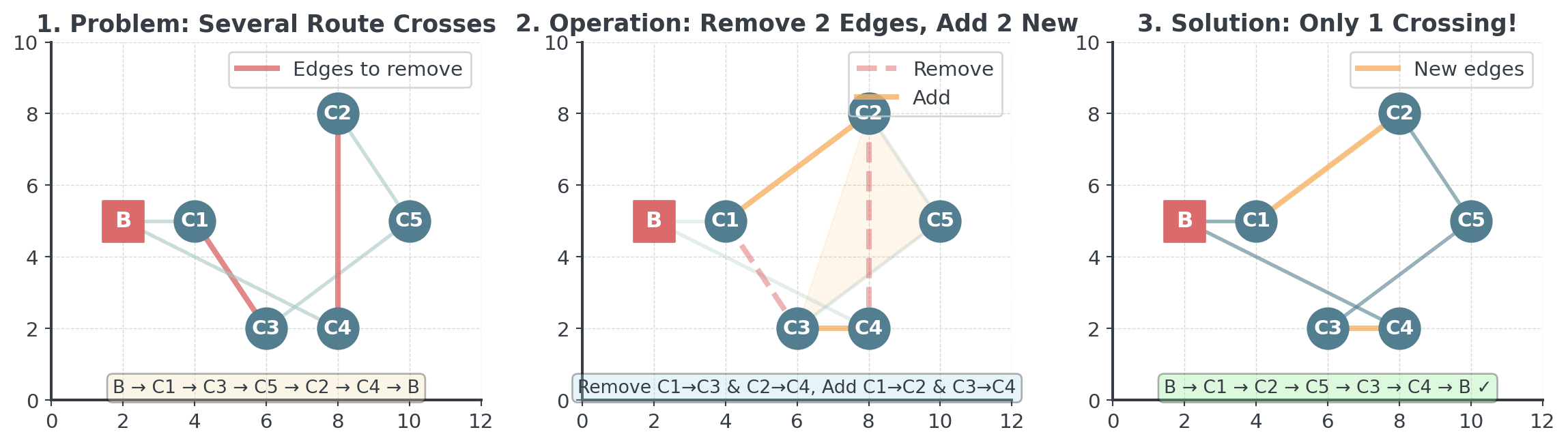
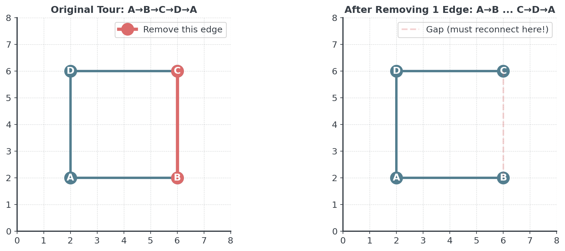
The 2-Opt Algorithm

Systematically improve routes by removing crossing paths.

. . .

The Idea: Take two edges and swap them (to uncross the route)

. . .

Example: Step-by-Step

Let’s see exactly how 2-opt fixes a crossing in a real route:

. . .

The Key Insight: When you reverse a segment between two crossing edges, you automatically eliminate the crossing and create a shorter route!

How 2-Opt Works

improved = True
while improved:
    improved = False
    best_distance = calculate_route_distance(route, distances)
    for i in range(len(route) - 1):
        for j in range(i + 2, len(route)):
            new_route = route[:i+1] + route[i+1:j+1][::-1] + route[j+1:]
            new_distance = calculate_route_distance(new_route, distances)
            if new_distance < best_distance:
                route = new_route
                best_distance = new_distance
                improved = True
                break
        if improved:
            break

. . .

The [::-1] reverses the segment, eliminating crossings!

2-Opt Applied

Let’s see how this changes the route!

. . .

. . .

Notice how 2-opt removed the crossing paths from our nearest neighbor solution, creating a more efficient route!

Common 2-Opt Bugs

Debug these scenarios you’ll encounter:

. . .

Bug 1: Infinite Loop

# WRONG: Forgot to update route
if new_distance < current_distance:
    improved = True  # But route never changes!

. . .

Bug 2: Missing Return to Start

# WRONG: Only measures cafe-to-cafe
total = sum(distances between stops)

. . .

Bug 3: Invalid Segment Reversal

# WRONG: Off-by-one error
new_route = route[:i] + route[i:j][::-1] + route[j:]

. . .

Fix: route[:i+1] + route[i+1:j+1][::-1] + route[j+1:]

What About 1-Opt?

. . .

Where 1-opt DOES work: In problems like knapsack (swap 1 item), assignment (reassign 1 person), or facility location (relocate 1 facility).

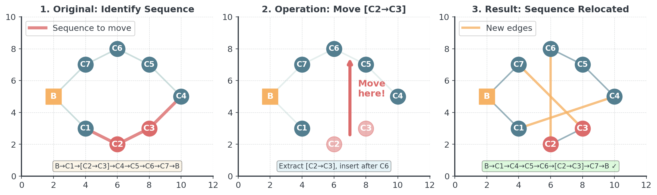
Or-Opt: Moving Sequences

Moves sequence of 1-3 consecutive cities to different position.

. . .

Moving a sequence can satisfy time constraints without breaking tour structure!

Beyond: k-Opt Neighborhoods

The k-opt family of improvements:

2-opt

Removes 2 edges
1 way to reconnect
n² combinations
Fast, good results

3-opt

Removes 3 edges
7 ways to reconnect
n³ combinations
Better but slower

Or-opt

Moves 1-3 nodes
Good for time windows
Specialized variant

. . .

Start with 2-opt (fast), use 3-opt if you have time! As k increases, solutions improve but computation time grows exponentially.

Local Optima

Convergence and Local Optima

When does local search stop? Why might it get stuck?

. . .

Convergence:

Algorithm stops when no neighboring solution is better

. . .

The Local Optimum Problem:

Algorithm can only “see” neighboring solutions
Might miss better solutions that require multiple changes
Like being stuck on a small hill when there’s a mountain nearby

. . .

Local search for improvement but does not guarantee global optimality.

The Local Optimum Trap

Imagine you’re a hiker dropped in foggy mountains at night…

Your Mission: Find the highest peak (global optimum)
Your Tool: An altimeter (objective function)
Your Vision: Only the ground at your feet (local neighborhood)

. . .

The Greedy Strategy: Always step uphill

. . .

Question: What happens when you reach the top of a small hill?

. . .

You’re stuck! Every step is downhill, but you might be on a tiny hill while a much larger moutain is nearby. This is the local optimum trap!

Visualizing Local Optima

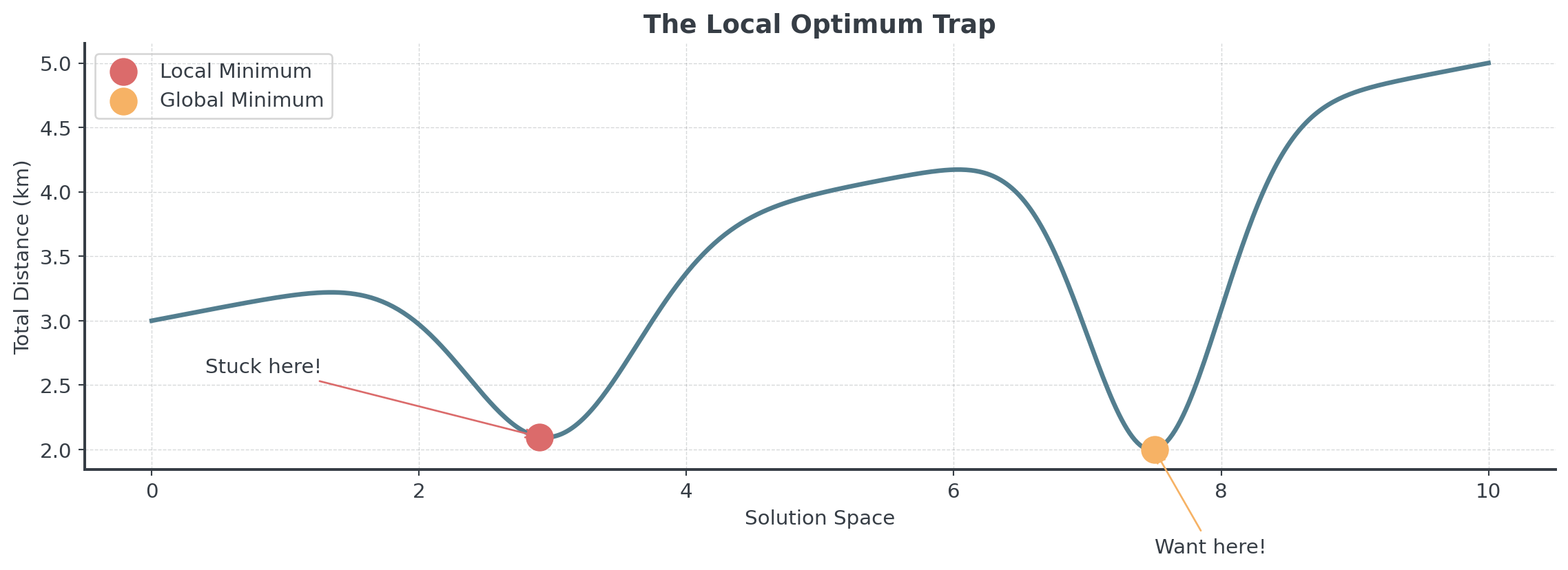
Here, the local minimum is already quite good, but we likely won’t reach the global optimum from here.

The Reality

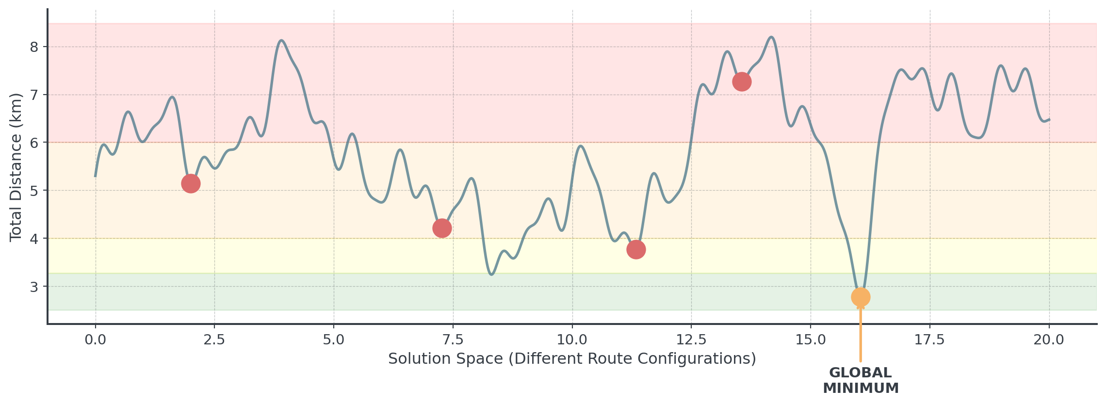
Real problems often have thousands of local optima!

. . .

The probability of finding the global optimum with simple local search is nearly zero!

Escaping Local Optima

Depending on the problem: Multi-Start Strategy!

Most local minima are much worse than the global optimum
The global minimum is sometimes isolated and hard to reach
Starting point dramatically affects final solution quality
Thus, start with different random solutions
Use different initial heuristics

. . .

No Free Lunch Theorem: There’s no universal “best” algorithm for all problems. What works great for routing might fail for scheduling. Always match your tool to your problem!

How Good is Good Enough?

Industry usage for delivery optimization

Method	Industry Use
Human intuition	Still common!
Start + 2-opt	Common practice
Advanced Meta	Sometimes practice
Exact (if possible)	Mostly research

. . .

A 10% improvement = millions in savings for large logistics companies. Even a 2-opt implementation could literally save a lot of money if not used yet!

Time Constraints

Time Windows

Remember our bakery? Some cafés open earlier than others!

. . .

Artisan Bakery’s Morning Schedule:

Bakery opens: 5:00 (van departs)
Early Birds (3 cafés): Must receive by 6:30
- Café Europa, Sunrise Bistro, Morning Glory
Standard (13 cafés): Must receive by 8:00

. . .

Question: Can we just find the shortest route?

. . .

The shortest route might deliver to early cafés last. Feasibility first, optimization second!

Time Windows: Practical Approach

Each location has a delivery time window:

Key Concepts:

Earliest time: When café opens
Latest time: Delivery deadline
Service time: Time to unload

. . .

Arrival Time = Previous departure + Travel time

. . .

Feasible route: All deadlines met
Infeasible route: At least one deadline missed (even if shortest!)

Time Windows: NN Modification

Modify greedy construction to prioritize early deadlines:

unvisited = set(range(len(locations))); route = []; current_time = start_time
while unvisited:
    # Find feasible neighbors (can reach before deadline)
    feasible = [i for i in unvisited
                if current_time + travel_time(current, i)
                    <= time_windows[i]['latest']]
    if not feasible:
        return None  # No feasible route exists!
    # Among feasible, choose most urgent
    next_stop = min(feasible, key=lambda i: (time_windows[i]['latest']))
    # Update state
    route.append(next_stop)
    unvisited.remove(next_stop)
    current_time += travel_time(current, next_stop) + service_time

2-Opt with Time Windows

Problem: 2-opt can break time feasibility!

. . .

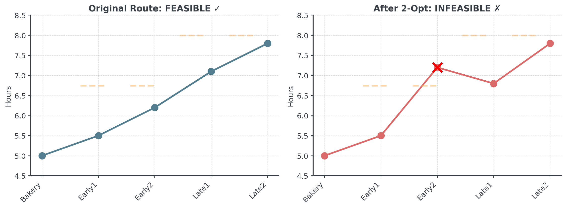
Early2 now arrives at 7:12 AM. Missed its 6:45 deadline by 27 minutes!

The Solution

Only accept swaps that maintain feasibility!

improved = True
while improved:
    improved = False
    for i in range(len(route) - 1):
        for j in range(i + 2, len(route)):
            new_route = route[:i+1] + route[i+1:j+1][::-1] + route[j+1:]
            # Check feasibility FIRST
            if not is_feasible(new_route, time_windows, start_time):
                continue  # Skip infeasible swaps
            # Among feasible swaps, take if shorter
            if calculate_distance(new_route) < calculate_distance(route):
                route = new_route
                improved = True
                break
        if improved:
            break

. . .

Feasibility is a hard constraint, distance is the objective.

Briefing

Choosing Your Algorithm

Different situations call for different approaches:

Situation	Best Approach	Why
Solution now	Nearest Neighbor	Lightning fast
Have seconds	NN + 2-opt	Good balance
Have minutes	Multi-start + 2-opt	Explore more options
Time windows	NN (early) + Or-opt	Preserves feasibility
Benchmark	3-opt or meta	Best solutions

. . .

Competition? Choose whatever you are comfortable with.

Implementation Pitfalls to Avoid

Common bugs that cost you time.

. . .

Forgetting return to bakery:

# WRONG
total = sum(distances between consecutive stops)
# RIGHT
total = sum(distances) + distance(last_stop, bakery)

. . .

Index confusion in 2-opt:

# The 2-opt swap reverses route[i+1:j+1], not route[i:j]

. . .

Modifying while iterating:

new_route = current_route.copy()  # Don't modify original

Escaping Local Optima

When local search gets stuck, we need clever escapes:

. . .

Advanced Techniques Coming:

Simulated Annealing: Sometimes accept worse moves
Genetic Algorithms: Combine good routes to make better ones
Tabu Search: Remember where you’ve been to avoid circles

. . .

Today’s local search foundation makes advanced methods possible!

Summary

Key Takeaways:

TSP is computationally hard (factorial growth)
Local search is a universal framework (4 pillars)
Greedy construction gives fast initial solutions
2-opt improves solutions iteratively
Multi-start helps escape local optima
Real constraints (time windows) add complexity
Two-phase approach: Build then improve!

Break!

Take 20 minutes, then we start the practice notebook

Next up: You’ll become Bean Counter’s route planner

Then: The Bakery competition