Notebook 9.1 - Metaheuristics: Beyond Local Optima
Management Science - Bean Counter’s European Expansion
Introduction
Welcome back, CEO! Bean Counter has grown to 1,000 cafés across Europe, and the Board just dropped a bombshell in your quarterly review:
The Distribution Crisis:
Current network: 50 distribution centers selected randomly 10 years ago
Annual logistics cost: €45 million (facility leases + delivery)
Competitors using optimization are 20% more efficient
Board mandate: Redesign the entire network or lose market share
You have 200 potential locations to choose from, and must select exactly 50 for new 10-year leases starting next quarter.
Your mission: Use advanced optimization to save €10+ million annually and prove that Bean Counter can compete in the age of AI.
WarningThe Stakes Are High
This is NOT a routing problem with a few trucks. This is a strategic infrastructure decision worth millions over the contract period. Simple methods will find good solutions. But metaheuristics can potentially find great solutions worth millions more.
NoteHow to Use This Tutorial
Work through each section in order. Write code where marked “YOUR CODE BELOW” and verify with the provided assertions. You’ll implement greedy, local search, simulated annealing, and genetic algorithms, the techniques you’ll need for the Restaurant Staffing Competition!
import numpy as npimport pandas as pdimport matplotlib.pyplot as pltfrom typing import List, Tuple, Setimport randomimport math# Set random seed for reproducibilitynp.random.seed(2025)random.seed(2025)print("Libraries loaded! Let's optimize Bean Counter's European distribution network.")
Libraries loaded! Let's optimize Bean Counter's European distribution network.
Section 1: Understanding the Distribution Network
Before we can optimize, we need to understand the scale and structure of Bean Counter’s challenge.
Bean Counter’s European Footprint
# DON'T CHANGE ANYTHING BELOW# Major European cities (simplified)european_cities = {'London': (51.5074, -0.1278, 120),'Paris': (48.8566, 2.3522, 95),'Berlin': (52.5200, 13.4050, 80),'Madrid': (40.4168, -3.7038, 75),'Rome': (41.9028, 12.4964, 65),'Amsterdam': (52.3676, 4.9041, 55),'Vienna': (48.2082, 16.3738, 50),'Barcelona': (41.3851, 2.1734, 60),'Munich': (48.1351, 11.5820, 45),'Hamburg': (53.5511, 9.9937, 40),'Milan': (45.4642, 9.1900, 55),'Prague': (50.0755, 14.4378, 35),'Brussels': (50.8503, 4.3517, 45),'Zurich': (47.3769, 8.5417, 40),'Copenhagen': (55.6761, 12.5683, 35),'Stockholm': (59.3293, 18.0686, 38),'Dublin': (53.3498, -6.2603, 32),'Lyon': (45.7640, 4.8357, 30),'Manchester': (53.4808, -2.2426, 28),'Lisbon': (38.7223, -9.1393, 42)}def generate_cafe_locations(cities_dict, total_cafes=1000):"""Generate café locations clustered around major European cities.""" cafes = [] cities_list =list(cities_dict.items())# Distribute cafés proportionally to city size total_weight =sum(weight for _, (_, _, weight) in cities_list)for city_name, (lat, lon, weight) in cities_list:# Number of cafés in this city's region n_cafes =int(total_cafes * weight / total_weight)# Generate cafés with some spread around city centerfor _ inrange(n_cafes):# Add random offset cafe_lat = lat + np.random.normal(0, 1.2) cafe_lon = lon + np.random.normal(0, 1.4) cafes.append((cafe_lat, cafe_lon))# Fill remaining cafés to reach exactly 1000whilelen(cafes) < total_cafes: city_name, (lat, lon, _) = random.choice(cities_list) cafe_lat = lat + np.random.normal(0, 0.7) cafe_lon = lon + np.random.normal(0, 0.7) cafes.append((cafe_lat, cafe_lon))return cafes[:total_cafes]# Generate café locationscafe_locations = generate_cafe_locations(european_cities)# Generate potential distribution center locations# (More concentrated near major cities, but with some strategic outliers)potential_centers = []cities_list =list(european_cities.items())for city_name, (lat, lon, weight) in cities_list:# More centers near bigger cities n_centers =max(5, int(200* weight /sum(w for _, (_, _, w) in cities_list)))for _ inrange(min(n_centers, 15)): # Cap per city center_lat = lat + np.random.normal(0, 2.0) center_lon = lon + np.random.normal(0, 2.0) potential_centers.append((center_lat, center_lon))# Ensure exactly 200 potential centerswhilelen(potential_centers) <200: city_name, (lat, lon, _) = random.choice(cities_list) center_lat = lat + np.random.normal(0, 0.7) center_lon = lon + np.random.normal(0, 0.7) potential_centers.append((center_lat, center_lon))potential_centers = potential_centers[:200]print(f"Bean Counter's European Network:")print(f" • {len(cafe_locations)} cafés requiring daily deliveries")print(f" • {len(potential_centers)} potential distribution center locations")print(f" • Must select exactly 50 centers for 10-year lease")print(f" • Each center: €500,000/year facility cost")print(f" • Each center serves exactly 20 cafés (balanced load)")print(f" • Delivery cost: €2 per km per day")print(f"\nTotal annual facility budget: €25,000,000")print("Delivery costs depend on your network design!")# DON'T CHANGE ANYTHING ABOVE
Bean Counter's European Network:
  • 1000 cafés requiring daily deliveries
  • 200 potential distribution center locations
  • Must select exactly 50 centers for 10-year lease
  • Each center: €500,000/year facility cost
  • Each center serves exactly 20 cafés (balanced load)
  • Delivery cost: €2 per km per day

Total annual facility budget: €25,000,000
Delivery costs depend on your network design!
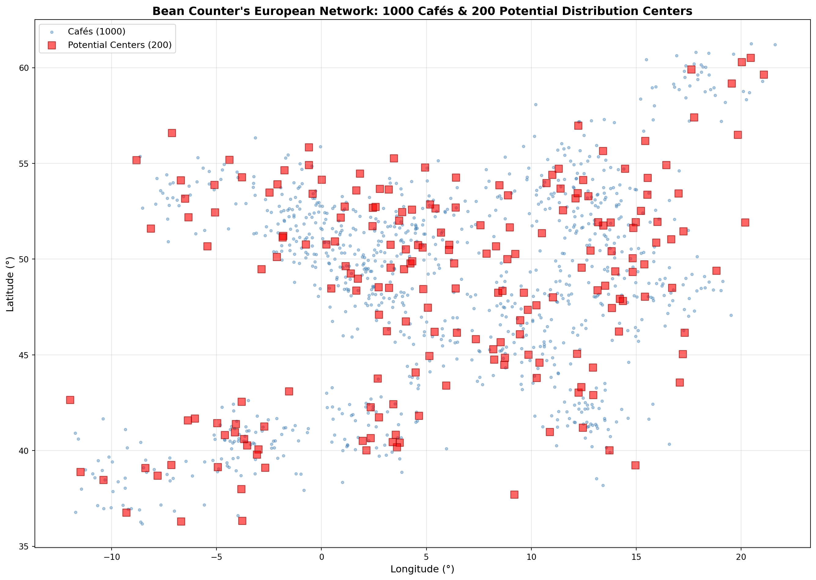
Visualizing the Network
Let’s see the geographic distribution of cafés and potential centers across Europe:
# Create visualization of Bean Counter's European networkplt.figure(figsize=(14, 10))# Plot caféscafe_lats = [loc[0] for loc in cafe_locations]cafe_lons = [loc[1] for loc in cafe_locations]plt.scatter(cafe_lons, cafe_lats, s=10, alpha=0.4, color='steelblue', label='Cafés (1000)')# Plot potential centerscenter_lats = [loc[0] for loc in potential_centers]center_lons = [loc[1] for loc in potential_centers]plt.scatter(center_lons, center_lats, s=80, alpha=0.6, color='red', marker='s', label='Potential Centers (200)', edgecolors='darkred', linewidth=1)plt.xlabel('Longitude (°)', fontsize=12)plt.ylabel('Latitude (°)', fontsize=12)plt.title("Bean Counter's European Network: 1000 Cafés & 200 Potential Distribution Centers", fontsize=14, fontweight='bold')plt.legend(fontsize=11)plt.grid(True, alpha=0.3)plt.tight_layout()plt.show()
Notice how cafés cluster around major European cities! This will be important for our optimization.
Calculating Geographic Distances
We’ll use the Haversine formula to calculate real distances between geographic coordinates.
TipThe Haversine Formula
For geographic coordinates (latitude, longitude), we can’t use simple Euclidean distance because Earth is a sphere!
The Haversine formula calculates great-circle distance:
Here it is already implemented, you just need to call it:
def haversine_distance(loc1: Tuple[float, float], loc2: Tuple[float, float]) ->float:"""Calculate distance in km between two (lat, lon) points using Haversine formula.""" lat1, lon1 = loc1 lat2, lon2 = loc2# Convert to radians lat1_rad = math.radians(lat1) lat2_rad = math.radians(lat2) lon1_rad = math.radians(lon1) lon2_rad = math.radians(lon2)# Differences dlat = lat2_rad - lat1_rad dlon = lon2_rad - lon1_rad# Haversine formula a = math.sin(dlat/2)**2+ math.cos(lat1_rad) * math.cos(lat2_rad) * math.sin(dlon/2)**2 c =2* math.asin(math.sqrt(a)) R =6371# Earth's radius in kmreturn R * c# Test the distance functiontest_dist = haversine_distance((51.5074, -0.1278), (48.8566, 2.3522)) # London to Parisprint(f"Example: London to Paris = {test_dist:.1f} km")test_dist2 = haversine_distance((52.5200, 13.4050), (48.2082, 16.3738)) # Berlin to Viennaprint(f"Example: Berlin to Vienna = {test_dist2:.1f} km")
Example: London to Paris = 343.6 km
Example: Berlin to Vienna = 523.5 km
Great! Now we can calculate real distances between any two locations in Europe.
Exercise 1.1: Implement the Network Cost Function with Balanced Allocation
This is the heart of the optimization, the function that determines if a network design is good or bad.
NoteWorking with Sets in Python
A set is an unordered collection with no duplicates:
unassigned = {1, 2, 3, 4, 5}unassigned.remove(3) # Remove element (error if not found)len(unassigned) # Number of elements3in unassigned # Check membership (fast!)
Why use sets here? Fast membership testing and removal. Perfect for tracking which cafés still need assignment!
TipBalanced Allocation Strategy
Key Innovation: Each center gets exactly 20 cafés (1000 ÷ 50 = 20)
Greedy Assignment Process:
For each selected center:
Find the 20 nearest unassigned cafés
Assign them to this center
Mark them as assigned
Sum up all delivery distances
Calculate total cost
Why this is better:
Always feasible - balanced load by construction
No capacity violations - each center gets exactly 20 cafés
Realistic - distribution territories are typically balanced
Simple - no penalty functions or feasibility checks needed
NoteBefore You Start
Here’s the implementation plan:
Loop through each selected center to assign its 20 cafés
For each center, calculate distances to ALL unassigned cafés using haversine_distance
Store results as tuples: [(distance1, cafe_idx1), (distance2, cafe_idx2), ...]
Sort the list by distance using .sort() (smallest first)
Take the first 20 using list slicing [:cafes_per_center]
Add distances to total and remove assigned cafés from the unassigned_cafes set
Hint: Loop for cafe_idx in unassigned_cafes: to build the distance list!
def calculate_network_cost(selected_centers: List[int], cafe_locs: List[Tuple[float, float]], center_locs: List[Tuple[float, float]], cafes_per_center: int=20) ->float:""" Calculate total annual cost using balanced greedy allocation. Args: selected_centers: List of indices (0-199) of selected centers cafe_locs: List of (lat, lon) tuples for cafés center_locs: List of (lat, lon) tuples for potential centers cafes_per_center: Number of cafés each center serves (default 20) Returns: total_cost: Total annual cost in € """# Fixed facility cost facility_cost =500_000*len(selected_centers)# Track which cafés have been assigned unassigned_cafes =set(range(len(cafe_locs))) total_daily_distance =0# Greedily assign cafés to each centerfor center_idx in selected_centers: center_loc = center_locs[center_idx]# Step 1: Calculate distances from this center to all unassigned cafés distances_to_unassigned = []for cafe_idx in unassigned_cafes: distance =# YOUR CODE - calculate distance using haversine_distance distances_to_unassigned.append((distance, cafe_idx))# Step 2: Sort by distance and take the nearest cafes_per_center cafés distances_to_unassigned.sort() nearest_cafes = distances_to_unassigned[:cafes_per_center]# Step 3: Add their distances to the total and mark as assignedfor distance, cafe_idx in nearest_cafes: total_daily_distance += distance unassigned_cafes.remove(cafe_idx)# Delivery cost: €2/km/day × 365 days delivery_cost = total_daily_distance *2*365 total_cost = facility_cost + delivery_costreturn total_cost
Code
# Test your cost function with a random networktest_centers = random.sample(range(200), 50)test_cost = calculate_network_cost(test_centers, cafe_locations, potential_centers)assert test_cost >25_000_000, "Cost should be > facility cost alone"assert test_cost <300_000_000, f"Cost seems too high: €{test_cost:,.0f}"print("Cost function working!")print(f"Random network cost: €{test_cost:,.0f}")print(f" Facility cost: €25,000,000")print(f" Delivery cost: €{test_cost -25_000_000:,.0f}")print(f"Note: Each center serves exactly 20 cafés - always balanced and feasible!")
Helper Function: Get Café-Center Assignments
No need to do anything here, we’ll use this function to determine which cafés are assigned to which centers for visualization:
def get_cafe_assignments(selected_centers: List[int], cafe_locs: List[Tuple[float, float]], center_locs: List[Tuple[float, float]], cafes_per_center: int=20) ->dict:""" Get the assignment of cafés to centers using the same greedy allocation as the cost function. Returns: Dictionary mapping center_idx -> list of assigned café indices """ unassigned_cafes =set(range(len(cafe_locs))) assignments = {}for center_idx in selected_centers: center_loc = center_locs[center_idx]# Calculate distances from this center to all unassigned cafés distances_to_unassigned = []for cafe_idx in unassigned_cafes: distance = haversine_distance(center_loc, cafe_locs[cafe_idx]) distances_to_unassigned.append((distance, cafe_idx))# Sort by distance and take the nearest cafes_per_center cafés distances_to_unassigned.sort() nearest_cafes = distances_to_unassigned[:cafes_per_center]# Record assignments assignments[center_idx] = [cafe_idx for _, cafe_idx in nearest_cafes]# Mark as assignedfor _, cafe_idx in nearest_cafes: unassigned_cafes.remove(cafe_idx)return assignments
Visualize Initial Random Solution
Let’s see what our random baseline looks like with connection lines:
# Visualize the initial random solutionplt.figure(figsize=(14, 10))# Get assignments for the random solutionrandom_assignments = get_cafe_assignments(test_centers, cafe_locations, potential_centers)# Plot connection lines first (so they appear behind markers)for center_idx, cafe_indices in random_assignments.items(): center_loc = potential_centers[center_idx]for cafe_idx in cafe_indices: cafe_loc = cafe_locations[cafe_idx] plt.plot([center_loc[1], cafe_loc[1]], [center_loc[0], cafe_loc[0]], 'gray', alpha=0.3, linewidth=1.5, zorder=1)# Plot all locations plt.scatter(center_lons, center_lats, s=80, alpha=0.1, color='red', marker='s', label='Potential Centers (200)', edgecolors='darkred', linewidth=1)# Plot caféscafe_lats = [loc[0] for loc in cafe_locations]cafe_lons = [loc[1] for loc in cafe_locations]plt.scatter(cafe_lons, cafe_lats, s=8, alpha=0.6, color='steelblue', label='Cafés (1000)', zorder=2)# Plot selected centersselected_lats = [potential_centers[i][0] for i in test_centers]selected_lons = [potential_centers[i][1] for i in test_centers]plt.scatter(selected_lons, selected_lats, s=150, alpha=1.0, color='red', marker='*', label='Random Centers (50)', edgecolors='darkred', linewidth=2, zorder=3)plt.xlabel('Longitude (°)', fontsize=12)plt.ylabel('Latitude (°)', fontsize=12)plt.title(f'Initial Random Solution: €{test_cost:,.0f}/year\n(Each line connects a café to its distribution center)', fontsize=14, fontweight='bold')plt.legend(fontsize=11)plt.grid(True, alpha=0.3)plt.tight_layout()plt.show()baseline_random_cost = test_cost # Save for comparison
Section 2: Greedy Construction - The Baseline
Let’s start with the simplest approach: pick the 50 centers that minimize total distance to cafés.
TipGreedy Algorithm Strategy
At each step, pick the center that gives the biggest immediate benefit:
Start with empty selection
For each of 50 iterations:
Try adding each remaining center
Calculate the cost with balanced allocation
Add the center with the lowest cost
Return final selection
Note: With balanced allocation, every solution is automatically feasible!
Exercise 2.1: Implement Greedy Center Selection
NoteBefore You Start
The greedy algorithm picks centers one at a time, always choosing the best addition:
Loop 50 times (one for each center to select)
For each candidate in the remaining centers:
Create temp_selection = selected + [candidate]
Calculate the cost if we selected this candidate
Track the candidate with the lowest cost
Add the best candidate to selected and remove from remaining
Key insight: This is expensive (trying ~150 centers × 50 times = 7,500 cost calculations), but it builds a good initial solution!
def greedy_center_selection(cafe_locs: List[Tuple[float, float]], center_locs: List[Tuple[float, float]], n_select: int=50) -> List[int]:""" Select distribution centers using greedy algorithm. Args: cafe_locs: Café locations center_locs: Potential center locations n_select: Number of centers to select Returns: List of selected center indices """ selected = [] remaining =set(range(len(center_locs)))print(f"Greedy selection: Selecting {n_select} centers...")for step inrange(n_select): best_center =None best_cost =float('inf')# Step 1: Try adding each remaining centerfor candidate in remaining:# Step 2: Create temporary selection with this candidate added temp_selection = selected + [candidate]# Step 3: Calculate cost with balanced allocation cost =# YOUR CODE - use calculate_network_cost# Step 4: Track if this is the best so farif cost < best_cost: best_cost =# YOUR CODE best_center =# YOUR CODE# Add the best center found selected.append(best_center) remaining.remove(best_center)if (step +1) %10==0:print(f" Selected {step +1}/{n_select} centers, current cost: €{best_cost:,.0f}")return selected
# Test greedy solutionassertlen(greedy_solution) ==50, "Should select exactly 50 centers"assertlen(set(greedy_solution)) ==50, "Should not select duplicates"assert greedy_cost < test_cost, f"Greedy should beat random baseline, got €{greedy_cost:,.0f}"baseline_random_cost = test_cost # Historical random selectiongreedy_savings = baseline_random_cost - greedy_costgreedy_improvement_pct = (greedy_savings / baseline_random_cost) *100print(f"Greedy algorithm complete!")print(f"Greedy network cost: €{greedy_cost:,.0f}")print(f"vs. Current random network: €{baseline_random_cost:,.0f}")print(f"Annual savings: €{greedy_savings:,.0f} ({greedy_improvement_pct:.1f}% improvement)")
Visualize the Greedy Solution
plt.figure(figsize=(14, 10))# Get assignments for the greedy solutiongreedy_assignments = get_cafe_assignments(greedy_solution, cafe_locations, potential_centers)# Plot connection lines first (so they appear behind markers)for center_idx, cafe_indices in greedy_assignments.items(): center_loc = potential_centers[center_idx]for cafe_idx in cafe_indices: cafe_loc = cafe_locations[cafe_idx] plt.plot([center_loc[1], cafe_loc[1]], [center_loc[0], cafe_loc[0]], 'blue', alpha=0.3, linewidth=1.5, zorder=1)# Plot all locations plt.scatter(center_lons, center_lats, s=80, alpha=0.1, color='red', marker='s', label='Potential Centers (200)', edgecolors='darkred', linewidth=1)# Plot all cafésplt.scatter(cafe_lons, cafe_lats, s=8, alpha=0.6, color='steelblue', label='Cafés', zorder=2)# Plot unselected centersunselected = [i for i inrange(200) if i notin greedy_solution]unselected_lats = [potential_centers[i][0] for i in unselected]unselected_lons = [potential_centers[i][1] for i in unselected]plt.scatter(unselected_lons, unselected_lats, s=40, alpha=0.2, color='gray', marker='s', label='Unselected Centers', zorder=2)# Plot selected centersselected_lats = [potential_centers[i][0] for i in greedy_solution]selected_lons = [potential_centers[i][1] for i in greedy_solution]plt.scatter(selected_lons, selected_lats, s=150, alpha=1.0, color='blue', marker='*', label='Greedy Selected (50)', edgecolors='black', linewidth=1, zorder=3)plt.xlabel('Longitude (°)', fontsize=12)plt.ylabel('Latitude (°)', fontsize=12)plt.title(f'Greedy Solution: €{greedy_cost:,.0f}/year ({greedy_improvement_pct:.1f}% improvement)\n(Blue lines show café-to-center assignments)', fontsize=14, fontweight='bold')plt.legend(fontsize=11)plt.grid(True, alpha=0.3)plt.tight_layout()plt.show()
WarningThe Greedy Trap
Greedy saved us some money! But greedy algorithms are short-sighted:
They make locally optimal choices
They never reconsider earlier decisions
They can’t escape suboptimal patterns
Can we do better?
Section 3: Local Search
Remember 2-opt swaps from the routing notebook? There, we improved routes by reversing segments. Here, we’ll use the same local search philosophy but with a different neighborhood:
Routing: Swap edges in a route (reverse a segment) Distribution Network: Swap centers in/out of the selection
The core idea remains: make small changes, keep improvements, stop at local optimum.
TipLocal Search
Core idea: Start with a solution, repeatedly make small changes that improve it.
The local search pattern:
Start with current solution
Generate a neighbor (slightly different solution)
If neighbor is better, keep it
Repeat until no improvement found
Problem: Gets stuck in local optima (can’t improve further, but not the global best)
Exercise 3.1: Implement the Swap Neighborhood
Create a neighbor by swapping one selected center with one unselected center.
NoteList Comprehensions for Filtering
Create new lists based on conditions in one line:
# Traditional approachunselected = []for i inrange(200):if i notin current_selection: unselected.append(i)# List comprehension (same result, cleaner!)unselected = [i for i inrange(200) if i notin current_selection]
Pattern:[expression for item in iterable if condition]
This is perfect for finding which centers are NOT currently selected!
NoteBefore You Start
Your implementation steps:
Find unselected centers: [i for i in range(n_centers) if i not in current_selection]
Pick a random position to remove from current_selection: random.randint(0, len(current_selection) - 1)
Pick a random center to add: random.choice(unselected)
Create a copy of current_selection and replace the element at the random index with the new center
Hint: Use .copy() to avoid modifying the original list!
def generate_swap_neighbor(current_selection: List[int], n_centers: int=200) -> List[int]:""" Generate a neighbor by swapping one selected center with one unselected. Args: current_selection: Current list of selected centers n_centers: Total number of potential centers Returns: New selection with one center swapped """# Get unselected centers unselected = [i for i inrange(n_centers) if i notin current_selection]# Pick random indices remove_idx = random.randint(0, len(current_selection) -1) add_center = random.choice(unselected)# Create new selection new_selection = current_selection.copy()# YOUR CODE: remove and add based on indicesreturn new_selection
Code
# Test swap functiontest_neighbor = generate_swap_neighbor(greedy_solution)assertlen(test_neighbor) ==50, "Neighbor should have 50 centers"assertlen(set(test_neighbor)) ==50, "No duplicates"assertlen(set(test_neighbor) &set(greedy_solution)) ==49, "Should differ by exactly 1 center"print("1-opt neighbor generation working!")print(f"Changed 1 center from the solution")
Exercise 3.2: Implement Local Search
Now implement the full local search algorithm.
NoteBefore You Start
Local search repeatedly tries to improve the current solution:
Try multiple neighbors each iteration (parameter: neighbors_per_iteration)
For each neighbor:
Generate it using generate_swap_neighbor(current)
Calculate its cost using calculate_network_cost(...)
If better than current, accept it immediately and break the inner loop
Track improvements: Increment counter when you accept a neighbor
Stop when stuck: If you try all neighbors and none improve, you’ve reached a local optimum
Key difference from greedy: Greedy builds from scratch; local search improves an existing solution!
def local_search(initial_solution: List[int], cafe_locs: List[Tuple[float, float]], center_locs: List[Tuple[float, float]], max_iterations: int=1000, neighbors_per_iteration: int=20) -> Tuple[List[int], float, int]:""" Improve a solution using local search. Args: initial_solution: Starting selection of centers cafe_locs: Café locations center_locs: Center locations max_iterations: Maximum improvement iterations neighbors_per_iteration: How many neighbors to try each iteration Returns: (best_solution, best_cost, num_improvements) """ current = initial_solution.copy() current_cost = calculate_network_cost(current, cafe_locs, center_locs) improvements =0print("Local search starting...")for iteration inrange(max_iterations): improved =False# Step 1: Try multiple neighbors per iterationfor _ inrange(neighbors_per_iteration):# Step 2: Generate neighbor neighbor =# YOUR CODE - use generate_swap_neighbor# Step 3: Evaluate neighbor neighbor_cost =# YOUR CODE - use calculate_network_cost# Step 4: If better, keep it and break inner loopif neighbor_cost < current_cost: current =# YOUR CODE current_cost =# YOUR CODE improvements +=1 improved =Truebreakif improved and (improvements %5==0):print(f" Iteration {iteration}: {improvements} improvements, cost: €{current_cost:,.0f}")ifnot improved:print(f"Local optimum reached after {iteration} iterations")breakreturn current, current_cost, improvements
# Run local search from greedy solutionls_solution, ls_cost, ls_improvements = local_search(greedy_solution, cafe_locations, potential_centers)
Code
# Test local searchassert ls_cost <= greedy_cost, "Local search shouldn't make solution worse"assert ls_improvements >=0, "Should track improvements"ls_savings = baseline_random_cost - ls_costls_improvement_pct = (ls_savings / baseline_random_cost) *100print(f"Local search complete!")print(f"Local search cost: €{ls_cost:,.0f}")print(f"vs. Greedy: €{greedy_cost:,.0f}")print(f"Additional savings: €{greedy_cost - ls_cost:,.0f}")print(f"Total vs. baseline: €{ls_savings:,.0f} ({ls_improvement_pct:.1f}% improvement)")print(f"Number of swaps: {ls_improvements}")
Visualize Local Search Solution
plt.figure(figsize=(14, 10))# Get assignments for the local search solutionls_assignments = get_cafe_assignments(ls_solution, cafe_locations, potential_centers)# Plot connection lines first (so they appear behind markers)for center_idx, cafe_indices in ls_assignments.items(): center_loc = potential_centers[center_idx]for cafe_idx in cafe_indices: cafe_loc = cafe_locations[cafe_idx] plt.plot([center_loc[1], cafe_loc[1]], [center_loc[0], cafe_loc[0]], 'mediumseagreen', alpha=0.3, linewidth=1.5, zorder=1)# Plot all locations plt.scatter(center_lons, center_lats, s=80, alpha=0.1, color='red', marker='s', label='Potential Centers (200)', edgecolors='darkred', linewidth=1)# Plot all cafésplt.scatter(cafe_lons, cafe_lats, s=8, alpha=0.6, color='steelblue', label='Cafés', zorder=2)# Plot selected centersselected_lats = [potential_centers[i][0] for i in ls_solution]selected_lons = [potential_centers[i][1] for i in ls_solution]plt.scatter(selected_lons, selected_lats, s=150, alpha=1.0, color='mediumseagreen', marker='*', label='Local Search Selected (50)', edgecolors='darkgreen', linewidth=1, zorder=3)plt.xlabel('Longitude (°)', fontsize=12)plt.ylabel('Latitude (°)', fontsize=12)plt.title(f'Local Search Solution: €{ls_cost:,.0f}/year ({ls_improvement_pct:.1f}% improvement)\n(Improved from Greedy by {ls_improvements} swaps)', fontsize=14, fontweight='bold')plt.legend(fontsize=11)plt.grid(True, alpha=0.3)plt.tight_layout()plt.show()
WarningThe Local Optimum Problem
Local search potentially finds a better solution than greedy, but this is not always the case as it can easily be stuck at a local optimum:
No single swap improves the solution
But a sequence of swaps (including temporary bad moves) might lead somewhere better
Like hiking: sometimes you must go downhill briefly to reach a higher peak
This is why we need metaheuristics!
Section 4: Simulated Annealing - Escaping Local Optima
Simulated Annealing (SA) is inspired by metallurgy: heating metal allows atoms to escape local patterns and find better arrangements as it cools.
Exercise 4.1: Implement the SA Acceptance Criterion
NoteBefore You Start
Idea: Sometimes accept worse solutions to escape local optima!
Implementation is straightforward:
If improvement (new_cost < current_cost): Always return True
If worse (new_cost >= current_cost):
Calculate delta = new_cost - current_cost
Calculate probability = math.exp(-delta / temperature)
Return True with that probability: random.random() < probability
Key insight: As temperature decreases, probability → 0, so SA becomes greedy!
TipAcceptance Probability - Concrete Examples
Scenario 1: Small cost increase, high temperature
Current: €40,000,000
Neighbor: €40,100,000 (€100K worse)
Temperature: T = 1,000,000
Delta = 100,000
Probability = exp(-100,000 / 1,000,000) = exp(-0.1) ≈ 90.5% → Often accept!
Probability = exp(-2,000,000 / 1,000,000) = exp(-2) ≈ 13.5% → Sometimes accept!
The pattern: Higher temperature → more exploration. Lower temperature → more exploitation.
def accept_move(current_cost: float, new_cost: float, temperature: float) ->bool:""" Decide whether to accept a move in simulated annealing. Args: current_cost: Current solution cost new_cost: Candidate solution cost temperature: Current temperature Returns: True if move should be accepted """if new_cost < current_cost:returnTrue# Always accept improvementselse:# Calculate acceptance probability delta =# YOUR CODE probability =# YOUR CODEreturn random.random() < probability
Code
# Test acceptance function# At high temp, should accept worse moves frequentlyhigh_temp_accepts =sum(accept_move(1000, 1100, temperature=500) for _ inrange(1000))assert high_temp_accepts >300, f"High temp should accept ~60% of moves, got {high_temp_accepts/10}%"# At low temp, should reject worse moveslow_temp_accepts =sum(accept_move(1000, 1100, temperature=10) for _ inrange(1000))assert low_temp_accepts <200, f"Low temp should accept <20% of moves, got {low_temp_accepts/10}%"# Always accept improvementsimprovements =sum(accept_move(1000, 900, temperature=100) for _ inrange(100))assert improvements ==100, "Should always accept improvements"print("Acceptance criterion working!")print(f"High temp (T=500): {high_temp_accepts/10:.1f}% acceptance for +€100 move")print(f"Low temp (T=10): {low_temp_accepts/10:.1f}% acceptance for +€100 move")
Exercise 4.2: Implement Simulated Annealing
Now put it all together! I will provide the cooling schedule, you implement the main loop.
NoteCooling Schedule
We’ll use geometric cooling: T_new = α × T_old
Initial temperature: T₀ = 10,000 (accept moves up to ~€10K worse initially)
Cooling rate: α = 0.995 (slow cooling for thorough exploration)
Stop when: T < 1 (essentially greedy behavior)
NoteBefore You Start
SA has TWO solutions to track (unlike local search which only tracks one):
Current solution: The solution we’re currently exploring (can get worse!)
Best solution: The best solution ever found (never gets worse)
Why both? We need to accept worse moves to escape local optima, but we don’t want to forget the best solution we’ve seen!
Your implementation steps:
Generate a neighbor using generate_swap_neighbor(current)
Calculate its cost using calculate_network_cost(...)
Use accept_move(current_cost, neighbor_cost, temperature) to decide
If accepted: Update current and current_cost (even if worse!)
Then check: If current is better than best ever, update best and best_cost
Critical: Track best separately from current!
def simulated_annealing(initial_solution: List[int], cafe_locs: List[Tuple[float, float]], center_locs: List[Tuple[float, float]], initial_temp: float=10000, cooling_rate: float=0.995, min_temp: float=1) -> Tuple[List[int], float, List[float]]:""" Optimize using simulated annealing. Args: initial_solution: Starting selection cafe_locs: Café locations center_locs: Center locations initial_temp: Starting temperature cooling_rate: Temperature multiplier each iteration min_temp: Stop when temperature reaches this Returns: (best_solution, best_cost, cost_history) """ current = initial_solution.copy() current_cost = calculate_network_cost(current, cafe_locs, center_locs) best = current.copy() best_cost = current_cost temperature = initial_temp cost_history = [current_cost] iteration =0print(f"SA starting from €{current_cost:,.0f} with T={initial_temp:,.0f}")while temperature > min_temp:for _ inrange(10): # 10 neighbors per temperature step# Step 1: Generate a neighbor neighbor =# YOUR CODE - use generate_swap_neighbor# Step 2: Calculate its cost neighbor_cost =# YOUR CODE - use calculate_network_cost# Step 3: Decide whether to accept using accept_move functionif accept_move(current_cost, neighbor_cost, temperature):# Step 4: Update current solution (even if worse!) current =# YOUR CODE current_cost =# YOUR CODE# Step 5: Track best ever foundif current_cost < best_cost: best =# YOUR CODE - use .copy()! best_cost =# YOUR CODE iteration +=1if iteration %200==0:print(f" Iteration {iteration}: T={temperature:.1f}, Current=€{current_cost:,.0f}, Best=€{best_cost:,.0f}")# Cool down temperature *= cooling_rate cost_history.append(current_cost)print(f"SA complete after {iteration} iterations")return best, best_cost, cost_history
# Run simulated annealing from greedy solutionsa_solution, sa_cost, sa_history = simulated_annealing(greedy_solution, cafe_locations, potential_centers)
Code
# Test SAassert sa_cost <= greedy_cost, "SA should improve upon starting solution"assertlen(sa_history) >100, "Should have run many iterations"sa_savings = baseline_random_cost - sa_costsa_improvement_pct = (sa_savings / baseline_random_cost) *100print(f"Simulated Annealing complete!")print(f"SA cost: €{sa_cost:,.0f}")print(f"vs. Local Search: €{ls_cost:,.0f}")print(f"vs. Greedy: €{greedy_cost:,.0f}")print(f"Additional savings over LS: €{ls_cost - sa_cost:,.0f}")print(f"Total vs. baseline: €{sa_savings:,.0f} ({sa_improvement_pct:.1f}% improvement)")
Visualize SA Evolution
fig, (ax1, ax2) = plt.subplots(1, 2, figsize=(15, 5))# Cost evolutionax1.plot(sa_history, alpha=0.7, linewidth=1, color='steelblue')ax1.axhline(y=greedy_cost, color='orange', linestyle='--', linewidth=1, label=f'Greedy: €{greedy_cost/1e6:.1f}M')ax1.axhline(y=ls_cost, color='green', linestyle='--', linewidth=1, label=f'Local Search: €{ls_cost/1e6:.1f}M')ax1.axhline(y=sa_cost, color='red', linestyle='--', linewidth=1, label=f'SA Best: €{sa_cost/1e6:.1f}M')ax1.set_xlabel('Iteration', fontsize=12)ax1.set_ylabel('Cost (€)', fontsize=12)ax1.set_title('Simulated Annealing Progress', fontsize=14, fontweight='bold')ax1.legend(fontsize=10)ax1.grid(True, alpha=0.3)# Temperature and acceptance visualization# Show when SA accepted worse moves (uphill moves)uphill_moves = [i for i inrange(1, len(sa_history)) if sa_history[i] > sa_history[i-1]]downhill_moves = [i for i inrange(1, len(sa_history)) if sa_history[i] <= sa_history[i-1]]ax2.scatter(downhill_moves, [sa_history[i] for i in downhill_moves], s=1, alpha=0.3, color='green', label='Improvements')ax2.scatter(uphill_moves, [sa_history[i] for i in uphill_moves], s=1, alpha=0.3, color='red', label='Accepted Worse Moves')ax2.set_xlabel('Iteration', fontsize=12)ax2.set_ylabel('Cost (€)', fontsize=12)ax2.set_title('SA Acceptance Behavior', fontsize=14, fontweight='bold')ax2.legend(fontsize=10)ax2.grid(True, alpha=0.3)plt.tight_layout()plt.show()print(f"\nAccepted {len(uphill_moves):,} worse moves (escaping local optima)")print(f"Made {len(downhill_moves):,} improvements")
Visualize SA Solution
plt.figure(figsize=(14, 10))# Get assignments for the SA solutionsa_assignments = get_cafe_assignments(sa_solution, cafe_locations, potential_centers)# Plot connection lines first (so they appear behind markers)for center_idx, cafe_indices in sa_assignments.items(): center_loc = potential_centers[center_idx]for cafe_idx in cafe_indices: cafe_loc = cafe_locations[cafe_idx] plt.plot([center_loc[1], cafe_loc[1]], [center_loc[0], cafe_loc[0]], 'gold', alpha=0.8, linewidth=1.5, zorder=1)# Plot all locations plt.scatter(center_lons, center_lats, s=80, alpha=0.1, color='red', marker='s', label='Potential Centers (200)', edgecolors='darkred', linewidth=1)# Plot all cafésplt.scatter(cafe_lons, cafe_lats, s=8, alpha=0.6, color='steelblue', label='Cafés', zorder=2)# Plot selected centersselected_lats = [potential_centers[i][0] for i in sa_solution]selected_lons = [potential_centers[i][1] for i in sa_solution]plt.scatter(selected_lons, selected_lats, s=150, alpha=1.0, color='gold', marker='*', label='SA Selected (50)', edgecolors='black', linewidth=1, zorder=3)plt.xlabel('Longitude (°)', fontsize=12)plt.ylabel('Latitude (°)', fontsize=12)plt.title(f'Simulated Annealing Solution: €{sa_cost:,.0f}/year ({sa_improvement_pct:.1f}% improvement)\n(Escaped local optima through controlled exploration)', fontsize=14, fontweight='bold')plt.legend(fontsize=11)plt.grid(True, alpha=0.3)plt.tight_layout()plt.show()print(f"Notice how SA found a different configuration than Local Search!")print(f"By accepting temporary worse moves, SA explored more of the solution space")print(f"This allowed it to escape local optima and find a better global solution")
Why SA beats Local Search:
Early exploration (high T): SA accepts worse moves, exploring far from greedy solution
Strategic descent (mid T): SA occasionally climbs small hills to find better valleys
Fine-tuning (low T): SA behaves like local search to polish the solution
The key: temporary bad decisions enable better long-term outcomes!
Section 5: CEO Decision Framework & Competition Connection
The Business Case
Let’s calculate the real financial impact, based on your results. Just execute the following code block:
Congratulations, CEO! You’ve mastered metaheuristics and saved Bean Counter millions! Your empire is now more efficient and profitable than ever before, thanks to your knowledge in management science. Your leadership has enabled Bean Counter to thrive in a competitive market, and has set the stage for even greater success!
What’s Next?
In the Restaurant Staffing Competition, you’ll:
Apply these algorithms to the scheduling problem
Optimize labor costs while meeting service requirements