Session 04 - Differentiation

Mathematics for Master Students

Author

Dr. Tobias Vlćek

Recap, Your Questions

Session 03 in a Nutshell

The roastery: demand \(D(p) = 1200 - 20p\) bags a week, cost \(C(q) = 200 + 5q\)
Revenue \(R(p) = 1200p - 20p^2\) peaks at the vertex €30
Profit \(\pi(p) = R(p) - C(D(p))\) peaks at €32.50; capacity of 500 bags pushes the price to €35
Composition \(C(D(p))\), the inverse \(D^{-1}(q) = 60 - \frac{q}{20}\), the chord test for convex and concave
Today: how fast does each of them change?

Common Issues in the Homework

One restriction forgotten: with \(\frac{\sqrt{x+1}}{x-2}\), both the root (\(x \geq -1\)) and the denominator (\(x \neq 2\)) restrict: collect every red flag, then intersect
Composition order: \((f \circ g)(x)\) means \(g\) acts first
The log-inequality flip: dividing by \(\ln 0.85 < 0\) flips the inequality. Dividing by a negative number always does

Which tasks gave you trouble? Bring them up now. We take the time to go through them before we move on to today’s topic.

Warm-Up: Average Cost of a Price

Question

The roastery’s average cost is \(A(q) = \frac{200}{q} + 5\) per bag, demand is \(D(p) = 1200 - 20p\). What is \(A(D(50))\), and which price must be excluded from \(A(D(p))\)? Type both.

Inside out: \(D(50) = 200\) bags, so \(A(D(50)) = \frac{200}{200} + 5 = 6\), €6 per bag
The division needs \(D(p) \neq 0\): \(1200 - 20p = 0\) at \(p = 60\), where nobody buys
The inner function must land where the outer one is defined: \(p = 60\) is out

Today’s Plan

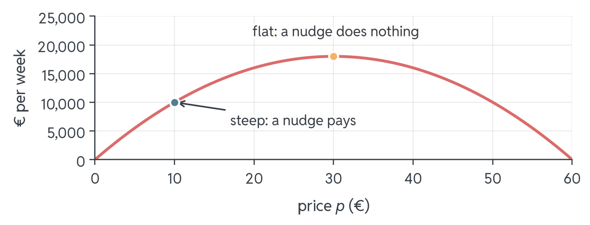
What does a €1 price rise add to the roastery’s revenue at €10, and at €30? Today: measure how steep a curve is at one point, then compute it in one line with the rules.

Rates of change: from a €1 nudge to the slope at one point
Differentiation rules: derivatives in one line, no limits needed
Second derivative: the chord test as a sign check
Marginal analysis: what the next bag costs and what it earns

Rates of Change

A €1 Price Rise

At price \(p\) the roastery earns \(R(p) = 1200p - 20p^2\) a week, Session 3's revenue parabola.

Question

The price goes up by €1. How much revenue does that add at \(p = 10\)? Guess in the chat.

\[R(11) - R(10) = 10780 - 10000 = 780\]

Now out loud: does a €1 rise at \(p = 30\) add more, less, or the same?

\[R(31) - R(30) = 17980 - 18000 = -20\]

Same €1 nudge, one curve: +€780 at €10, −€20 at €30. Why?

The Same Nudge, Different Effects

Revenue parabola over the price with two marked points: at p = 10 the curve is steep, so a small price rise pays, and at p = 30, the top of the curve, it is flat, so a small price rise changes almost nothing.

Steep at €10, flat at €30: the answer is the steepness of the curve where we stand.

The Average Rate of Change

The €780 was revenue change per €1 of price; divide by the step \(h\) for the difference quotient (the average rate of change):

\[\frac{R(10 + h) - R(10)}{h} \quad\longrightarrow\quad \frac{f(a+h) - f(a)}{h}\]

Change in output over change in input
How much does \(f\) change as the input moves from \(a\) to \(a + h\)?
A line gives the same slope \(m\) for every \(a\) and \(h\)
The curve does not: from \(p = 10\), \(h = 1\) gives \(780\). What does \(h = 10\) give?

Geometry: The Secant Line

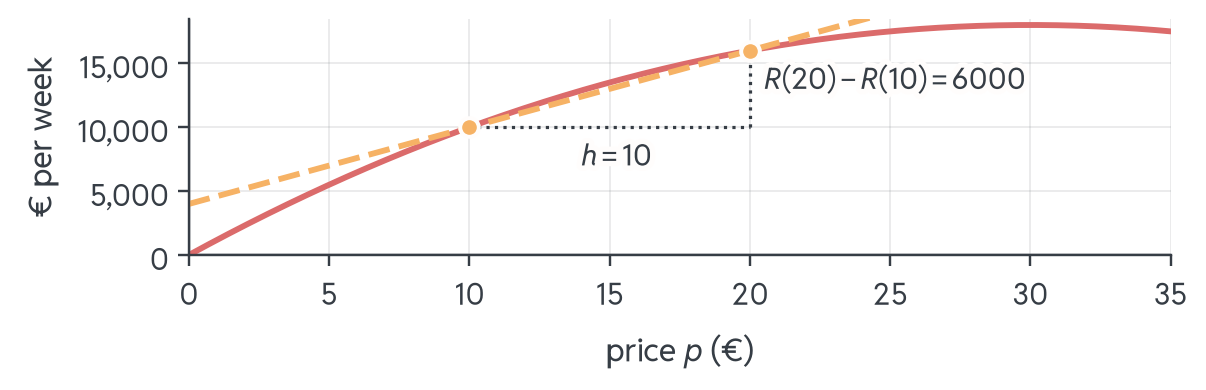
Revenue curve with a dashed secant line through its points at p = 10 and p = 20. Dotted lines mark the step between them: h = 10 across and R(20) − R(10) = 6000 up.

The difference quotient is the slope of the secant line through \((10, R(10))\) and \((20, R(20))\): \(\frac{16000 - 10000}{10} = 600\) euros of revenue per euro of price.

Your Turn: Find the Secant Slope

Question

For \(R(p) = 1200p - 20p^2\), what is the difference quotient from \(p = 10\) to \(p = 15\)? Type the number in the chat.

\[\frac{R(15) - R(10)}{5} = \frac{13500 - 10000}{5} = 700\]

A step of \(10\) gave \(600\) and a step of \(5\) gives \(700\): as the second price closes in on €10, the slope climbs. Where does it stop?

Zoom In Until the Curve Is Straight

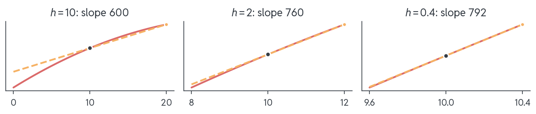
Three zooms on the revenue curve around p = 10, each with the dashed secant through p = 10 and p = 10 + h. For h = 10 the curve bends away from the secant (slope 600), for h = 2 much less (slope 760), and for h = 0.4 curve and secant look like the same straight line (slope 792).

Zoom in on a smooth curve and it turns straight; the secant stops tilting. That straight line is the tangent at \(p = 10\), and its slope is the rate of change right at \(p = 10\).

Letting \(h\) Shrink

The secant slope of revenue, \(\frac{R(p+h) - R(p)}{h}\), at the two prices from the start:

\(h\)	\(10\)	\(5\)	\(1\)	\(0.1\)	\(0.01\)
at \(p = 10\)	\(600\)	\(700\)	\(780\)	\(798\)	\(799.8\)
at \(p = 30\)	\(-200\)	\(-100\)	\(-20\)	\(-2\)	\(-0.2\)

As \(h\) shrinks toward \(0\), the slopes settle on \(800\) and \(0\)
We write \(\lim_{h \to 0}\) for “the value it settles on as \(h\) shrinks toward \(0\)”
That is all the limit theory we need in this tutorial

The Derivative

The derivative of \(f\) at \(a\) is the instantaneous rate of change:

\[f'(a) = \lim_{h \to 0} \frac{f(a+h) - f(a)}{h}\]

Geometric reading: slope of the tangent line at \((a, f(a))\)
Business reading: \(R'(10) = 800\): at €10, revenue reacts at €800 per euro of price
Taken at every point: a new function \(f'\), the derivative of \(f\)
Positive \(f'\): increasing; negative \(f'\): decreasing
Session 3's revenue: \(R' > 0\) below €30, \(R' < 0\) above

Your Turn: Read the Sign

Question

You are told \(f'(a) = -3\). What does that say?

(a) \(f\) is falling at \(a\), slope \(-3\)	(b) The value \(f(a)\) equals \(-3\)
(c) \(f\) has a minimum at \(a\)	(d) \(f\) drops by exactly \(3\) up to \(a + 1\)

(a): the derivative is a slope, and a negative slope means the graph falls at \(a\).

(d) is only approximately right, and only for a nearly straight graph: the tangent slope describes the trend at \(a\), not a whole unit further on. (b) confuses the value with the slope.

Notation for Derivatives

All of these mean the same thing:

Notation	Read as
\(f'(x)\)	“\(f\) prime of \(x\)”
\(\dfrac{df}{dx}\)	“derivative of \(f\) with respect to \(x\)”
\(\dfrac{d}{dx} f(x)\)	“\(\frac{d}{dx}\) applied to \(f(x)\)”

\(\frac{df}{dx}\) deliberately looks like a difference quotient: it reminds you where the derivative comes from. We mostly write \(f'(x)\); when the letters are not \(f\) and \(x\) (e.g. \(R(p)\)), the \(\frac{dR}{dp}\) form says with respect to what: € of revenue per € of price.

Your Turn: Average vs Derivative

Question

A courier van covers 150 km in 2 hours. Halfway through, a speed camera clocks it at 90 km/h. Which statement is right?

(a) The camera is wrong: the van averaged 75 km/h	(b) Both hold: 90 km/h is an average, 75 km/h a derivative
(c) Both hold: 75 km/h is an average, 90 km/h a derivative	(d) Just one can hold: a van has one speed per trip

(c): \(\frac{150}{2} = 75\) km/h is a difference quotient; the camera’s 90 km/h is the instantaneous rate, the derivative of distance
Both can hold: the average smooths out faster and slower stretches

Where Zooming Fails

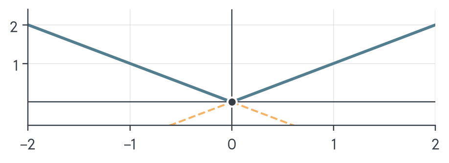
Graph of the absolute value |x|, a V with its corner at the origin. Dashed lines continue each arm through the corner, one with slope −1 and one with slope +1: two different directions, so there is no single tangent at 0.

Zoom into \(|x|\) at \(0\) as far as you like: the corner stays a corner. Secants from the left settle on \(-1\), from the right on \(+1\), so there is no single tangent and no derivative at \(0\)
A function has a derivative (is differentiable) only where it is smooth: no kinks, no jumps; tiered shipping tariffs jump at their breakpoints

Differentiation Rules

Constants and the Power Rule

For \(x^2\) the difference quotient simplifies:

\[\frac{(x+h)^2 - x^2}{h} = \frac{2xh + h^2}{h} = 2x + h \;\to\; 2x \quad \text{as } h \to 0\]

The pattern holds for every power:

Power rule: \((x^n)' = n x^{n-1}\), exponent down front, then one less
Constants: \(f(x) = c\) never changes, so \(f'(x) = 0\)

The Power Rule for All Exponents

One rule decides what negative and fractional powers mean: multiplying adds exponents, \(x^a \cdot x^b = x^{a+b}\).

\(x^{-1} \cdot x = x^0 = 1\), so \(x^{-1} = \dfrac{1}{x}\) and \(\left(\dfrac{1}{x}\right)' = -1 \cdot x^{-2} = -\dfrac{1}{x^2}\)
\(x^{1/2} \cdot x^{1/2} = x^1\), so \(x^{1/2} = \sqrt{x}\) and \(\left(\sqrt{x}\right)' = \dfrac{1}{2} x^{-1/2} = \dfrac{1}{2\sqrt{x}}\) (\(x > 0\))

Rewrite as a power, differentiate, translate back. Sanity check: \(\frac{1}{x}\) falls, so its slope must be negative ✓

Your Turn: Apply the Power Rule

Question

Let \(f(x) = x^4\). What is \(f'(2)\)? Type the number.

\[f'(x) = 4x^3, \qquad f'(2) = 4 \cdot 8 = 32\]

Common Mistake

\(f'(2) = 4 \cdot 2^4 = 64\) forgets to reduce the exponent. Exponent down front and one less on top.

Bonus: A Negative Power

Differentiate \(g(x) = \dfrac{1}{x^2}\):

\[g(x) = x^{-2}, \qquad g'(x) = -2x^{-3} = -\frac{2}{x^3}\]

Sums and Constant Multiples

\[(c \cdot f)'(x) = c \cdot f'(x) \qquad (f + g)'(x) = f'(x) + g'(x)\]

Together: differentiate term by term, constants tag along
Example, a print shop whose cost bends upward, unlike the roastery’s straight line: \(C(q) = 0.5q^2 + 10q + 200\)
\(C'(q) = 0.5 \cdot 2q + 10 + 0 = q + 10\)
The fixed costs \(200\) vanish: they do not react to producing one unit more

Your Turn: Term by Term

Question

A cost function is \(C(q) = 0.1q^2 + 4q + 50\). What is \(C'(20)\)? Type the number.

\[C'(q) = 0.2q + 4, \qquad C'(20) = 4 + 4 = 8\]

At \(20\) units, cost grows at €8 per unit, while the fixed cost \(50\) has disappeared from \(C'\) entirely: it never reacts to output.

Revenue Is a Rectangle

Revenue \(R(p) = p \cdot D(p)\): price along the bottom, bags sold up the side. Raise \(p = 10\) by \(h\):

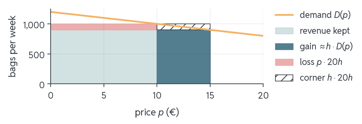
Revenue as a rectangle under the falling demand line: price along the bottom, bags sold up the side. Raising the price from 10 by h adds a tall gain strip on the right, cuts a flat loss strip off the top, and leaves a small hatched corner where the two strips meet.

Gains on bags still sold, losses on bags no longer sold, and a corner that shrinks like \(h^2\).

The Product Rule

\[R'(p) = \underbrace{1 \cdot D(p)}_{\text{gain}} + \underbrace{p \cdot D'(p)}_{\text{loss}} = (1200 - 20p) - 20p = 1200 - 40p\]

The \(1\) is \(p' = 1\): price’s own rate of change with respect to itself
In general: \((f \cdot g)'(x) = f'(x)\,g(x) + f(x)\,g'(x)\), each factor takes its turn to change

The Quotient Rule

Session 3 saw the roastery’s average cost \(A(q) = (200 + 5q)/q\) settle towards €5. Does it fall with every bag?

\[\left(\frac{f}{g}\right)'(x) = \frac{f'(x)\,g(x) - f(x)\,g'(x)}{\left(g(x)\right)^2}\]

Like the product rule, but a growing denominator shrinks the quotient: hence the minus, and the order matters
Here \(f = 200 + 5q\) and \(g = q\), so \(f' = 5\) and \(g' = 1\)
\(A'(q) = \dfrac{5 \cdot q - (200 + 5q) \cdot 1}{q^2} = -\dfrac{200}{q^2} < 0\): falls with every bag

Machines in a Row: Rates Multiply

The price sets the bags, the bags the cost: \(p \xrightarrow{\;D\;} q \xrightarrow{\;C\;} C(D(p))\)

Question

With \(D(p) = 1200 - 20p\) and \(C(q) = 200 + 5q\), the price rises by €1. How does the weekly cost change? Type the number.

€1 more: \(20\) bags fewer, each saves €5: cost changes by \((-20) \cdot 5 = -100\), €100 less per week
Check by composing: \(C(D(p)) = 200 + 5(1200 - 20p) = 6200 - 100p\), slope \(-100\) ✓
Chain rule: rates multiply, \(\frac{d}{dp}\,C(D(p)) = C'(q) \cdot D'(p)\)

The Chain Rule

When the outer function curves, its rate depends on what the inner one delivers. A warehouse: stock \(q(t) = 30 + 4t\) pallets after \(t\) weeks, storage cost \(H(q) = 0.2q^2\) in €.

Stock rate \(q'(t) = 4\) pallets per week; cost rate \(H'(q) = 0.4q\) € per pallet, read at the current stock
At \(t = 5\): \(q = 50\), so cost rises at \(0.4 \cdot 50 \cdot 4 = 80\), €80 per week
In general: \(\left(f(g(x))\right)' = f'(g(x)) \cdot g'(x)\), outer derivative at the inner value, times the inner derivative
Bracket to a power: \((x^2+1)^3\): outer \((\cdot)^3\) gives \(3(x^2+1)^2\), inner \(x^2 + 1\) gives \(2x\), so \(\left((x^2+1)^3\right)' = 6x(x^2+1)^2\)

Your Turn: Spot the Missing Factor

Question

What is the derivative of \((3x + 2)^5\)?

(a) \(5(3x + 2)^4\)	(b) \(15(3x + 2)^4\)
(c) \(5 \cdot 3^4\)	(d) \(15x\,(3x + 2)^4\)

(b): outer derivative \(5(3x+2)^4\), times the inner derivative \(3\).

(a) forgot the inner factor, (c) differentiated the bracket away, (d) invented an \(x\): the inner derivative of \(3x + 2\) is the constant \(3\), nothing more. Forgetting the inner factor is the classic chain-rule slip.

Your Turn: Pick the Rule

Question

Which rules differentiate (i) \((5x+1)^4\), (ii) \(x^3(2x - 7)\), (iii) \(\frac{x}{x^2+1}\), in that order?

(a) power · product · quotient	(b) chain · chain · quotient
(c) chain · product · power	(d) chain · product · quotient

(d) is right:

(i) Chain rule, outer \((\cdot)^4\): derivative \(4(5x+1)^3 \cdot 5 = 20(5x+1)^3\)
(ii) Product rule: \(3x^2(2x - 7) + x^3 \cdot 2 = 8x^3 - 21x^2\), or expand first: same result
(iii) Quotient rule: \(\left(\frac{x}{x^2+1}\right)' = \frac{1 \cdot (x^2 + 1) - x \cdot 2x}{(x^2 + 1)^2} = \frac{1 - x^2}{(x^2 + 1)^2}\)

Which Base Has Slope 1?

Every \(b^x\) passes through \((0, 1)\). How steep is it there? \(2^x\) has slope \(0.69\), \(3^x\) has \(1.10\): which base has slope exactly \(1\)?

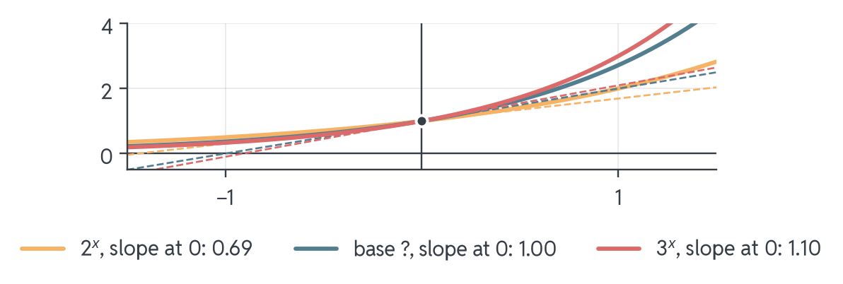
Three exponential curves through the point (0, 1), each with its dashed tangent there: base 2 with slope 0.69, base 3 with slope 1.10, and between them a curve with an unnamed base whose slope is exactly 1.00.

Between base \(2\) (0.69) and base \(3\) (1.10) sits the base with slope exactly \(1\): Euler’s number \(e \approx 2.718\).

Derivatives of \(e^x\) and \(a^x\)

\(\left(e^x\right)' = e^x\): the slope equals the height, everywhere
Other bases, chain rule on \(a^x = e^{x \ln a}\): \(\left(a^x\right)' = a^x \ln a\); the 0.69 in the plot is \(\ln 2\)
With the chain rule: \(\left(e^{3x}\right)' = 3e^{3x}\)
Growth, Session 3's \(K(t) = K_0 e^{rt}\): the chain rule gives \(K'(t) = r\,K(t)\)
The €1000 reserve at \(r = 0.05\) grows at 5% of what it holds
Only base \(e\) makes the factor exactly the rate \(r\): that is why growth models use \(e\)

The Derivative of \(\ln x\)

\(\ln\) is \(e^x\) mirrored, and a slow climber: \(\left(\ln x\right)' = \dfrac{1}{x}\)
Sanity check: at \((1, 0)\) the slope is \(1\); by \(x = e\) the curve has climbed just one unit, and the slope is down to \(1/e\)

Your Turn: Exponential and Log

Question

Differentiate \(f(x) = e^{2x}\) and \(g(x) = \ln(5x)\). Which pair is right?

(a) \(2e^{2x}\) and \(\frac{1}{x}\)	(b) \(2e^{2x}\) and \(\frac{5}{x}\)
(c) \(2x\,e^{2x}\) and \(\frac{1}{x}\)	(d) \(e^{2x}\) and \(\frac{1}{5x}\)

(a) is right: \(f'(x) = e^{2x} \cdot 2 = 2e^{2x}\): inner derivative \(2\)
\(g'(x) = \dfrac{1}{5x} \cdot 5 = \dfrac{1}{x}\): the \(5\) cancels
No surprise: \(\ln(5x) = \ln 5 + \ln x\); \(\ln 5\)’s derivative is zero
(b) multiplied, not cancelled; (c) invented an \(x\); (d) missed both factors

The Rule Table

Building blocks

\(f(x)\)	\(f'(x)\)
\(c\)	\(0\)
\(x^n\)	\(n x^{n-1}\)
\(e^x\)	\(e^x\)
\(a^x\)	\(a^x \ln a\)
\(\ln x\)	\(\frac{1}{x}\)

Combinations

Rule	Formula
Constant multiple	\((c f)' = c f'\)
Sum	\((f + g)' = f' + g'\)
Product	\((f g)' = f'g + f g'\)
Quotient	\(\left(\frac{f}{g}\right)' = \frac{f'g - f g'}{g^2}\)
Chain	\((f(g))' = f'(g) \cdot g'\)

The Second Derivative

Does the Slope Itself Change?

Session 3's advertising curve: \(S(a) = 100\sqrt{a}\) extra bags from a budget \(a\) (in €1000). Each extra €1000 added \(+100\), \(+41\), \(+32\), \(+27\).

The slope tells the same story, \(S'(a) = \dfrac{50}{\sqrt{a}}\):

budget \(a\)	\(1\)	\(4\)	\(9\)
slope \(S'(a)\)	\(50\)	\(25\)	\(16.7\)

Question

The slope falls as the budget grows. How would you measure how fast it falls?

Differentiating Twice

The slope \(f'\) is again a function, so differentiate again:

\[f''(x) = \left(f'\right)'(x) \qquad \text{also written } \frac{d^2 f}{dx^2}\]

\(f'\) reports how fast \(f\) changes; \(f''\) how fast the slope changes
Advertising: \(S''(a) = -\dfrac{25}{a^{3/2}} < 0\), so the slope shrinks at every budget: diminishing returns
A cubic: \(f(x) = x^3 - 3x\), \(f'(x) = 3x^2 - 3\), \(f''(x) = 6x\)
Third, fourth, \(\dots\) derivatives exist too: for us, two is all we need

Your Turn: Differentiate Twice

Question

Let \(f(x) = 2x^3 - 5x\). What is \(f''(3)\)? Type the number.

\[f'(x) = 6x^2 - 5, \qquad f''(x) = 12x, \qquad f''(3) = 36\]

Positive: at \(x = 3\) the slope is increasing; the graph bends upward, convex there. The next slide makes that reading official.

Convex or Concave? Ask \(f''\)

Session 3's chord test becomes a sign check on an interval:

\(f''(x) \geq 0\) on the interval \(\Rightarrow\) convex: the slope never falls, every chord lies on or above the graph
\(f''(x) \leq 0\) on the interval \(\Rightarrow\) concave: the slope never rises, every chord lies on or below the graph
\(f(x) = x^2\): \(f''(x) = 2 \geq 0\), convex everywhere
\(S''(a) < 0\): the advertising curve is concave, diminishing returns certified

Reading \(f\), \(f'\) and \(f''\) Together

Same cubic, three views. Watch the sign of the right panel and how the left curve bends.

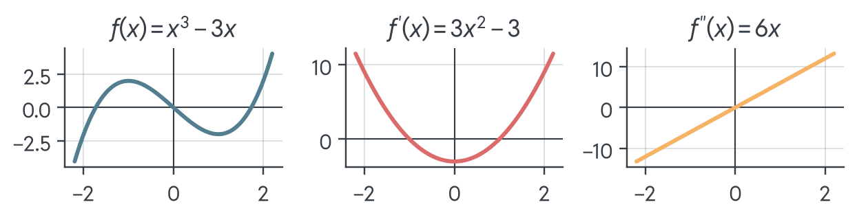
Three panels for the same cubic. Left: f(x) = x³ − 3x bends downward for x below 0 and upward for x above 0. Middle: its slope 3x² − 3, a parabola with its lowest point at x = 0. Right: the second derivative 6x, a line through the origin, negative left of 0 and positive right of it.

For \(x < 0\): \(f'' < 0\): slope falling, \(f\) bends downward (concave)
For \(x > 0\): \(f'' > 0\): slope rising, \(f\) bends upward (convex)
At \(x = 0\) the bend switches, an inflection point; Session 5 turns these signs into an optimisation tool

Your Turn: What If \(C''(q) > 0\)?

Question

The print shop’s cost \(C(q) = 0.5q^2 + 10q + 200\) has \(C'(q) = q + 10\) and \(C''(q) = 1\). What does \(C'' > 0\) say about the next unit?

(a) Total cost falls once output is large	(b) Each extra unit costs the same amount
(c) Each extra unit costs more than the last	(d) The fixed cost grows with every unit

(c): the slope \(C'\) keeps rising, so every further unit is dearer. The cost curve is convex.

(b) holds only for a straight cost line such as the roastery’s, €5 per bag. (a) confuses the curvature with the slope: \(C' > 0\) for all \(q \geq 0\), so cost only rises. (d) is wrong because the fixed €200 never changes.

Marginal Analysis

Marginal Cost

The last question already used it. What does the next unit cost?

Roastery, \(C(q) = 200 + 5q\): bag 401 costs \(C(401) - C(400) = 5\), i.e. €5, at any volume: the slope
Print shop, \(C(q) = 0.5q^2 + 10q + 200\): the curve steepens, so the answer depends on \(q\)
With \(h = 1\) in the difference quotient: \(C(q+1) - C(q) \approx C'(q)\)
One unit is a small nudge next to hundreds produced, so the tangent slope is an excellent stand-in
Economists call \(C'(q)\) the marginal cost: the instantaneous rate at which cost grows, approximately the cost of one more unit

Your Turn: The 101st Unit

Question

The print shop again, \(C(q) = 0.5q^2 + 10q + 200\). Approximately what does the 101st unit cost? Type the number.

\[C'(100) = 100 + 10 = 110 \qquad \text{so about €110}\]

Exact check: \(C(101) - C(100) = 6310.5 - 6200 = 110.5\). The tangent slope misses by 50 cents, and it is far quicker than the subtraction.

Marginal Revenue

What does the next bag earn? That question asks about bags, so revenue counted in bags gets its own name, \(\tilde R(q)\). Session 3's inverse \(D^{-1}(q) = 60 - \frac{q}{20}\) prices the \(q\)-th bag:

\[\tilde R(q) = q \cdot D^{-1}(q) = 60q - \frac{q^2}{20}, \qquad \tilde R'(q) = 60 - \frac{q}{10} \ \text{(€ per bag)}\]

At 400 bags, \(\tilde R'(400) = 20\): bag 401 earns about €20 and costs €5, so sell it
At 600 bags (\(p = 30\)), \(\tilde R'(600) = 0\): revenue’s flat top

Marginal Revenue vs Marginal Cost

Marginal revenue falls with \(q\): every extra bag needs a lower price
The next bag pays off while \(\tilde R'(q) > C'(q)\); where the two meet lies the profit-maximal output, Session 5 proves it
Where do \(60 - \frac{q}{10}\) and \(5\) meet? Hold that thought for Session 5

Closing

Key Takeaways

A €1 rise at \(p = 10\) adds €780; \(R'(10) = 800\) is the tangent’s slope, the limit of the difference quotient
Zoom into a smooth graph and it turns straight; kinks and jumps (\(|x|\) at \(0\), tiered tariffs) never do
Revenue is a rectangle, \(R' = D + p\,D'\); along a chain rates multiply: \(-20\) bags per € times €5 per bag

Key Takeaways: \(e\), \(f''\), Margins

\(e^x\) is the exponential whose slope equals its height: the reserve grows at exactly \(r\) times itself
Each extra €1000 of advertising adds less: \(S'' < 0\), concave; \(f'' \geq 0\) convex, \(f'' \leq 0\) concave
Bag 401 costs €5 and earns about €20; at €30, \(R' = 0\). Is the profit tangent flat at €32.50?

That’s it for today.

Any Questions?

Until the Next Session

Work through the Tasks: the drilling happens there, with worked solutions
Check yourself with the Self-Test quiz
Keep the Cheatsheet next to you: the rule table lives on it: ten lines for every function in Session 3's gallery
Note down anything unclear: we start next session with your questions

When differentiating, name the structure first: sum, product, quotient or chain? The right rule follows automatically.

Preview: Session 05: Optimisation

Central question: where is a function largest or smallest?
Profit slope = revenue slope − cost slope: \(\pi'(p) = 1300 - 40p\). Where is it flat?
The recipe: set \(f'\) to zero (flat tangent) and ask \(f''\) whether it is a peak or a valley
Session 3's €32.50 and €35 again, this time from the derivative
Today’s rules become the toolkit: best price, output, order quantity

See you there, and bring your questions!

Literature & Further Reading

These sessions cover the essentials: textbooks offer more depth and practice
Start with Sydsæter et al. (2012) or Jacques (2015); full recommendations on the tutorial’s literature page

Jacques, Ian. 2015. Mathematics for Economics and Business. 8th ed. Always Learning. Pearson.

Sydsæter, Knut, Peter J. Hammond, and Arne Strøm. 2012. Essential Mathematics for Economic Analysis. 4th ed. Pearson.