Session 06 - Systems of Linear Equations
Mathematics for Master Students
Recap, Your Questions
Session 05 in a Nutshell
- FOC: the roastery’s profit hill is flat where \(\pi'(p) = -40p + 1300 = 0\): €32.50, found without the vertex formula
- SOC: \(\pi'' = -40 < 0\) makes it a peak; a flat tangent alone can be a saddle (\(x^3\) at \(0\)), and \(f'' = 0\) says nothing (\(x^4\))
- Boundaries: €32.50 needs 550 bags: capacity allows 500, so \(p \geq 35\); profit falls on \([35, 60]\) and the boundary wins, €35
Session 05: Two Business Rules
- MR = MC: the print shop stops at \(q = 45\), where the next unit earns €55 and costs €55
- Balance: the print shop’s average cost bottoms out at €30 (\(q = 20\)); the warehouse orders \(200\) at a time: falling and rising costs equal, \(q^* = \sqrt{2DK/h}\)
- Today: several conditions at once, and where their lines cross
Common Issues in the Homework
- Endpoints forgotten (P4): on \([0, 3]\) the interior stationary point gave the minimum \(-11\); the true maximum \(f(0) = 5\) sits at the boundary: the endpoints are always candidates
- The cap ignored (P5): the FOC returned \(q = 60\), but the plant makes at most \(50\). Since \(\pi'(50) = 10 > 0\), profit is still rising: the best feasible output is \(q = 50\), not \(60\)
- A sign slip in the SOC: \(f''(x^*) < 0\) is a maximum (concave), not a minimum: check the sign before naming the type
Which tasks gave you trouble? Bring them up now. We take the time to work through them before moving on.
Warm-Up: Where Do Lines Cross?
NoteQuestion
The roastery sells \(D(p) = 1200 - 20p\) bags a week at price \(p\) and can roast at most \(500\). Write “sell exactly 500” as two lines, \(q = 1200 - 20p\) and \(q = 500\). At which price do they cross?
- \(1200 - 20p = 500 \;\Rightarrow\; 20p = 700 \;\Rightarrow\; p = 35\)
- Session 5's boundary price: the capacity line crosses the demand line at €35
- Two equations, two unknowns \(p\) and \(q\), one crossing point: a system of linear equations
Today’s Plan
The roastery’s house blend must hit a weight and a cost target at once: how many kg of each bean? Today: turn every target into an equation, then find the point that meets them all.
- Setting up a system: two targets, two lines, one crossing point
- Demand and supply: a market as two equations in two unknowns
- Gaussian elimination: the workshop’s three products and three limits
- How many solutions? and what if there is not exactly one
Setting Up a System
One Blend, Two Targets
The roastery’s house blend mixes a base bean at €4/kg and a premium bean at €8/kg. This week’s batch must weigh 20 kg and cost €5 per kg on average, the €5 per (1 kg) bag in its cost \(C(q) = 200 + 5q\).
NoteQuestion
How many kg of each bean?
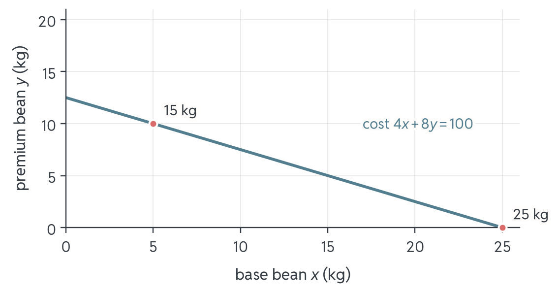
With \(x\) kg base and \(y\) kg premium, the weight target is \(x + y = 20\) and the cost target is \(4x + 8y = 20 \cdot 5 = 100\) (€100 for 20 kg). Does the cost target on its own fix the blend?
One Equation, a Line of Blends
One condition in two unknowns is a whole line: every dot costs €100, but the batch weighs 25 or 15 kg. The cost target alone cannot choose.
Your Turn: On the Cost Line?
NoteQuestion
Which blend costs exactly €100?
| (a) \(8\) kg base, \(9\) kg premium | (b) \(9\) kg base, \(8\) kg premium |
| (c) \(10\) kg base, \(10\) kg premium | (d) \(12\) kg base, \(5\) kg premium |
(b): \(4 \cdot 9 + 8 \cdot 8 = 36 + 64 = 100\) ✓. The others cost €104, €120 and €88.
But (b) weighs only \(17\) kg, and (c) weighs the right \(20\) kg at the wrong price. Each target alone has many answers; we need both at once.
A System Pins It Down
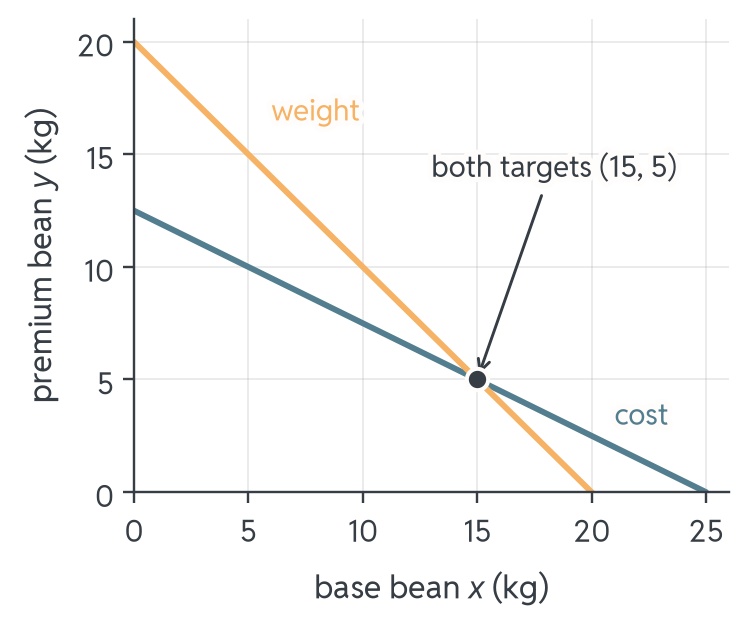
- A system of linear equations asks several conditions to hold at the same time: a solution lies on every line
- The solutions are the intersection of the weight line \(x + y = 20\) and the cost line \(4x + 8y = 100\), just as Session 2's feasible set was the intersection of the constraints
Method 1: Substitution
Solve one equation for one variable, then substitute into the other.
- From the weight equation: \(x = 20 - y\)
- Put that into the cost equation: \(4(20 - y) + 8y = 100\)
- Expand: \(80 - 4y + 8y = 100 \;\Rightarrow\; 80 + 4y = 100\)
- So \(4y = 20\) and \(y = 5\)
- Back-substitute: \(x = 20 - 5 = 15\)
- Solution: \(15\) kg base and \(5\) kg premium, the crossing from the plot
Method 2: Elimination
Scale the equations so one variable cancels when you subtract.
- Multiply the weight equation by \(4\): \(4x + 4y = 80\)
- Subtract it from the cost equation: \[(4x + 8y) - (4x + 4y) = 100 - 80 \;\Rightarrow\; 4y = 20 \;\Rightarrow\; y = 5\]
- Back-substitute: \(x + 5 = 20 \;\Rightarrow\; x = 15\)
- Always check: \(15 + 5 = 20\) ✓ and \(4 \cdot 15 + 8 \cdot 5 = 60 + 40 = 100\) ✓
Your Turn: Two Trucks
NoteQuestion
Two trucks carry \(10\) pallets in total, and the first carries \(4\) more than the second: \(x + y = 10, \quad x - y = 4\). Ideas for \((x, y)\)?
- Add the equations: \(2x = 14 \Rightarrow x = 7\)
- Back-substitute: \(7 + y = 10 \Rightarrow y = 3\)
- Check: \(7 - 3 = 4\) ✓, so \((x, y) = (7, 3)\)
Adding instead of subtracting is elimination too: whichever move makes a variable cancel.
What Makes an Equation Linear?
Every condition today drew a straight line. Which equations do that? An equation is linear when every unknown appears on its own, to the first power, nothing more exotic.
- Linear: \(2x + 3y = 13\), or \(x + 2y + 2z = 16\), a weighted sum of the variables
- Not linear: \(x^2 + y = 4\) (a square), \(xy = 6\) (a product), \(\sqrt{x} + y = 1\) (a root), \(2^x = 8\) (an exponent)
Your Turn: Linear or Not?
NoteQuestion
Is \(\frac{x}{2} = 7 - 3y\) a linear equation in \(x\) and \(y\)?
- Yes: move \(3y\) across and it reads \(\frac{1}{2}x + 3y = 7\)
- The quick test: it has the shape (number)\(\cdot x\) + (number)\(\cdot y =\) number
- A fraction as a coefficient changes nothing; only what happens to the unknowns counts
Demand and Supply
Market Equilibrium
At which price is there neither a queue nor unsold stock?
From here on \(D(p)\) is a whole market’s demand, not the roastery’s:
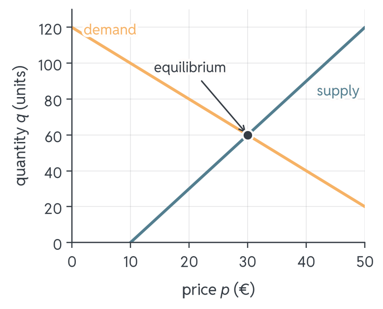
- Demand: \(D(p) = 120 - 2p\): buyers want less as the price rises
- Supply: \(S(p) = 3p - 30\): sellers offer more as the price rises
- Equilibrium is the price where quantity wanted equals quantity offered, both at once, a \(2 \times 2\) system (two equations, two unknowns)
Supply Meets Demand
Look where the lines cross: about €30.
Your Turn: Above the Equilibrium
NoteQuestion
The price is set at €40, above the equilibrium of about €30. Do sellers offer more than buyers want (a surplus, excess supply) or less (a shortage, excess demand)?
- Demand at €40: \(120 - 80 = 40\); supply at €40: \(3 \cdot 40 - 30 = 90\)
- Sellers offer \(90\) but buyers want only \(40\), a surplus of \(50\) units
- Above equilibrium there is surplus (excess supply); price pressure pushes back down toward €30
- Below it the reverse: a shortage (excess demand)
Solving for Equilibrium
The picture says about €30. Elimination makes it exact: move the \(p\)-terms of \(q = 120 - 2p\) and \(q = 3p - 30\) to the left: \[q + 2p = 120, \qquad q - 3p = -30.\]
- Subtract the second from the first: \(5p = 150 \;\Rightarrow\; p = 30\)
- Back-substitute: \(q = 120 - 2(30) = 60\)
- Equilibrium: price €30, quantity \(60\) units
- Check the supply side: \(3(30) - 30 = 60\) ✓
- Or substitute directly: \(120 - 2p = 3p - 30 \;\Rightarrow\; 150 = 5p\), same \(p\)
Your Turn: Find the Equilibrium
NoteQuestion
Another market: demand \(D(p) = 100 - p\), supply \(S(p) = 2p - 20\). What is the equilibrium price?
\[100 - p = 2p - 20 \quad \Rightarrow \quad 120 = 3p \quad \Rightarrow \quad p = 40\]
Check the supply side: \(2 \cdot 40 - 20 = 60\) ✓. Price €40, quantity \(q = 100 - 40 = 60\) units.
Gaussian Elimination
Three Products, Three Limits
The workshop makes \(x\), \(y\) and \(z\) units of three products this week:
| per unit | \(x\) | \(y\) | \(z\) | available |
|---|---|---|---|---|
| Packaging (units) | 1 | 1 | 1 | 9 |
| Labour (h) | 1 | 2 | 2 | 16 |
| Machine (h) | 2 | 1 | 3 | 17 |
Every resource must be used up, so each row is one condition: \(x + y + z = 9\), \(x + 2y + 2z = 16\), \(2x + y + 3z = 17\).
NoteQuestion
Method 2 turned two unknowns into one. What would you do with three?
Your Turn: Read It Bottom-Up
NoteQuestion
A system arrives in this shape: \(x + 2y + z = 10, \quad y - z = 1, \quad z = 2\). What is \(x\)?
- Bottom: \(z = 2\)
- Middle: \(y - 2 = 1 \Rightarrow y = 3\)
- Top: \(x + 6 + 2 = 10 \Rightarrow x = 2\)
Solution \((2, 3, 2)\). Each equation has one unknown fewer than the one above: a triangular form, solved from the bottom up.
Knock Out \(x\)
Eq. 1: \(x + y + z = 9\)
Eq. 2: \(x + 2y + 2z = 16\)
Eq. 3: \(2x + y + 3z = 17\)
Method 2 again, twice: subtract multiples of the first equation so that \(x\) cancels.
- Eq. 2 − Eq. 1: \((x + 2y + 2z) - (x + y + z) = 16 - 9 \;\Rightarrow\; y + z = 7\)
- Eq. 3 − 2 · Eq. 1: \((2x + y + 3z) - (2x + 2y + 2z) = 17 - 18 \;\Rightarrow\; -y + z = -1\)
- What is left is a \(2 \times 2\) system in \(y\) and \(z\), the shape of Two Trucks
Equal minus equal stays equal, so no solution is lost. Adding Eq. 1 back undoes the step, so no new one appears.
Drop the Letters
We copied \(x\), \(y\), \(z\) and every plus sign again and again, yet only the numbers changed. Keep just the numbers, the augmented matrix (\(R_1, R_2, R_3\) name the rows):
\[\left[\begin{array}{ccc|c} 1 & 1 & 1 & 9 \\ 1 & 2 & 2 & 16 \\ 2 & 1 & 3 & 17 \end{array}\right] \;\xrightarrow[\;R_3 \,\to\, R_3 - 2R_1\;]{\;R_2 \,\to\, R_2 - R_1\;}\; \left[\begin{array}{ccc|c} 1 & 1 & 1 & 9 \\ 0 & 1 & 1 & 7 \\ 0 & -1 & 1 & -1 \end{array}\right]\]
Each row is an equation and the bar stands for the equals sign. The step we just did by hand is now one arrow. No matrix algebra, pure bookkeeping.
Your Turn: One Row Operation
NoteQuestion
Rows \(R_1 = (1, 2, -1 \,|\, 3)\) and \(R_2 = (2, 5, 1 \,|\, 9)\). Compute \(R_2 - 2R_1\).
\[\begin{aligned}(2, 5, 1 \,|\, 9) - 2 \cdot (1, 2, -1 \,|\, 3) &= (2 - 2,\; 5 - 4,\; 1 + 2 \,|\, 9 - 6) \\ &= (0, 1, 3 \,|\, 3)\end{aligned}\]
WarningCommon Mistake
\(1 - 2 \cdot (-1) = 1 + 2 = 3\), not \(-1\): subtracting a negative adds.
Three Allowed Moves
Whatever is fair for equations is fair for rows. Three row operations:
- Swap two rows (e.g. when the top row has no \(x\))
- Scale a row by a non-zero number (multiply both sides of one equation)
- Add a multiple of one row to another (subtracting \(2R_1\) adds \(-2R_1\): how we knocked out \(x\))
One test covers all three: can you undo it? Swap back, divide back, subtract back. A move you can undo neither loses nor creates a solution: the solution set stays the same.
Your Turn: Which Move Is Illegal?
NoteQuestion
Which of these is not an allowed row operation?
| (a) Swap \(R_1\) and \(R_3\) | (b) Replace \(R_2\) by \(R_2 - 3R_1\) |
| (c) Multiply \(R_3\) by \(0\) | (d) Divide \(R_2\) by \(2\) |
(c): multiplying by \(0\) turns the row into \(0 = 0\), and nothing multiplies it back. The condition is gone for good, and the solution set can grow.
Swap, divide by \(2\) and subtract \(3R_1\) can all be undone, so the solution set stays the same.
Clear the Second Column
Rows 2 and 3 read \(y + z = 7\) and \(-y + z = -1\), the Two Trucks shape. Add them, then divide by 2:
\[\left[\begin{array}{ccc|c} 1 & 1 & 1 & 9 \\ 0 & 1 & 1 & 7 \\ 0 & -1 & 1 & -1 \end{array}\right] \;\xrightarrow[\;R_3 \,\to\, R_3 / 2\;]{\;R_3 \,\to\, R_3 + R_2\;}\; \left[\begin{array}{ccc|c} 1 & 1 & 1 & 9 \\ 0 & 1 & 1 & 7 \\ 0 & 0 & 1 & 3 \end{array}\right]\]
- \(R_3 + R_2\): \((0,-1,1\,|\,{-1}) + (0,1,1\,|\,7) = (0,0,2\,|\,6)\)
- \(R_3 / 2\): \((0,0,2\,|\,6) \div 2 = (0,0,1\,|\,3)\)
Back-Substitution
The workshop’s system is now in triangular form, like the one from the start of this section. Read it from the bottom up:
\[x + y + z = 9, \qquad y + z = 7, \qquad z = 3\]
- Bottom row: \(z = 3\)
- Middle row: \(y + 3 = 7 \;\Rightarrow\; y = 4\)
- Top row: \(x + 4 + 3 = 9 \;\Rightarrow\; x = 2\)
- Solution: \((x, y, z) = (2, 4, 3)\)
Always Verify
Plug the triple \((2, 4, 3)\) back into the original three equations:
- Packaging: \(2 + 4 + 3 = 9\) ✓
- Labour: \(2 + 8 + 6 = 16\) ✓
- Machine: \(4 + 4 + 9 = 17\) ✓
Make \(2\) of \(x\), \(4\) of \(y\), \(3\) of \(z\): every resource used to the last unit.
WarningCommon Mistake
When you apply a row operation, act on the whole row, the right-hand side included. Subtracting \(2R_1\) from \(R_3\) but forgetting to also do \(17 - 2 \cdot 9 = -1\) silently corrupts the whole solve.
Your Turn: Check a Rival Plan
- Packaging: \(x + y + z = 9\)
- Labour: \(x + 2y + 2z = 16\)
- Machine: \(2x + y + 3z = 17\)
NoteQuestion
A colleague proposes the plan \((x, y, z) = (3, 3, 3)\) instead. Which resource does it exceed?
| (a) Packaging (\(9\)) | (b) Labour (\(16\) h) |
| (c) Machine (\(17\) h) | (d) None, it also works |
Only One Plan Fits Exactly
(c), with \((3, 3, 3)\):
| resource | used | available | verdict |
|---|---|---|---|
| Packaging | \(3 + 3 + 3 = 9\) | \(9\) | ✓ |
| Labour | \(3 + 6 + 6 = 15\) | \(16\) | 1 h idle |
| Machine | \(6 + 3 + 9 = 18\) | \(17\) | exceeded |
A linear system with a unique solution has exactly one plan that uses every resource fully. Any other plan breaks a limit, leaves something idle, or, like \((3, 3, 3)\), both.
Gaussian Elimination in Four Steps
- Write the augmented matrix: coefficients left, right-hand sides right of the bar
- Eliminate forward: knock out \(x\) below the top row, then \(y\) below the second, until the triangular form appears
- Back-substitute: read the triangular system from the bottom row up
- Verify: plug the solution into the original equations
Work on one column at a time and write every intermediate matrix down. Elimination fails through slips, not through difficulty.
How Many Solutions?
Two Lines on a Page
NoteQuestion
Two straight lines on a page. How many points can they share? Could it be exactly two?
- One: they cross: a unique solution (every example so far)
- None: they never meet: the conditions contradict each other
- Infinitely many: they are the same line: one condition is redundant
- Never exactly two: two shared points already fix the whole line
Two Lines: No Solution
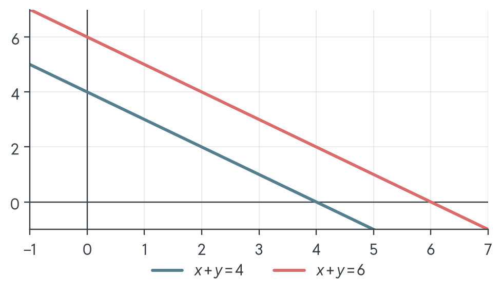
\(x + y = 4\) and \(x + y = 6\) are parallel, same slope, different heights. They never meet, so no pair \((x, y)\) satisfies both.
Two Lines: Infinitely Many
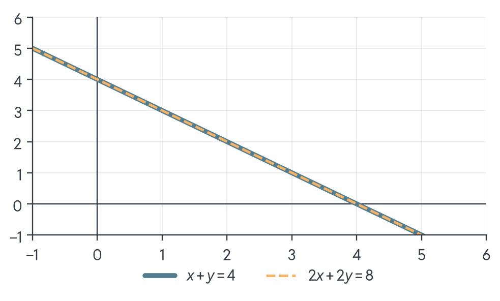
\(2x + 2y = 8\) is just \(x + y = 4\) doubled, the same line. Every point on it solves both; there are infinitely many solutions.
Parameterising the Free Case
When one equation adds nothing new, we describe all solutions with a free parameter.
For \(x + y = 4\) with a redundant partner:
- Let \(y = t\) be free, any real number
- Then \(x = 4 - t\)
- Solution set: \((x, y) = (4 - t,\; t)\), one point for each \(t\)
- E.g. \(t = 0 \to (4, 0)\), \(t = 1 \to (3, 1)\), \(t = 4 \to (0, 4)\)
Your Turn: Pick a Solution
NoteQuestion
The solution set is \((x, y) = (4 - t,\; t)\). Which point belongs to it?
| (a) \((5, 1)\) | (b) \((1, 3)\) |
| (c) \((3, 2)\) | (d) \((2, 4)\) |
(b): \(t = 3\) gives \((4 - 3, 3) = (1, 3)\). Equivalently, \(1 + 3 = 4\) ✓.
The quick test is the original equation \(x + y = 4\): the other three sum to \(6\), \(5\) and \(6\).
Planes Instead of Lines
With three unknowns, each equation is a plane in space, but the same three fates return:
- Unique: two walls and the floor meet in one corner, like the workshop’s \((2, 4, 3)\)
- None: floor and ceiling never meet; or a tent: every two of its three planes meet, yet no point lies on all three
- Infinitely many: the pages of an open book share the spine, a whole line of solutions (or a whole plane)
The New Machine: 20 Hours
The workshop replaces its machine. The new one needs \(2, 3, 3\) hours per product, and \(20\) hours are available: \(2x + 3y + 3z = 20\)
\[\left[\begin{array}{ccc|c} 1 & 1 & 1 & 9 \\ 1 & 2 & 2 & 16 \\ 2 & 3 & 3 & 20 \end{array}\right] \;\xrightarrow[\;R_3 \,\to\, R_3 - 2R_1\;]{\;R_2 \,\to\, R_2 - R_1\;}\; \left[\begin{array}{ccc|c} 1 & 1 & 1 & 9 \\ 0 & 1 & 1 & 7 \\ 0 & 1 & 1 & 2 \end{array}\right]\]
A Contradiction Appears
\[\left[\begin{array}{ccc|c} 1 & 1 & 1 & 9 \\ 0 & 1 & 1 & 7 \\ 0 & 1 & 1 & 2 \end{array}\right] \;\xrightarrow{\;R_3 \,\to\, R_3 - R_2\;}\; \left[\begin{array}{ccc|c} 1 & 1 & 1 & 9 \\ 0 & 1 & 1 & 7 \\ 0 & 0 & 0 & -5 \end{array}\right]\]
- The last row reads \(0 = -5\): no plan uses every resource exactly
- Why: machine row = packaging + labour, \((2, 3, 3) = (1, 1, 1) + (1, 2, 2)\)
- Using both fully needs \(9 + 16 = 25\) machine hours, not \(20\)
- The tent: every two of the three planes meet, all three never do
The New Machine: 25 Hours
With \(25\) hours instead, the value that packaging and labour already imply:
\[\left[\begin{array}{ccc|c} 1 & 1 & 1 & 9 \\ 1 & 2 & 2 & 16 \\ 2 & 3 & 3 & 25 \end{array}\right] \;\xrightarrow[\;R_3 \,\to\, R_3 - 2R_1\;]{\;R_2 \,\to\, R_2 - R_1\;}\; \left[\begin{array}{ccc|c} 1 & 1 & 1 & 9 \\ 0 & 1 & 1 & 7 \\ 0 & 1 & 1 & 7 \end{array}\right]\]
A Row Vanishes
\[\left[\begin{array}{ccc|c} 1 & 1 & 1 & 9 \\ 0 & 1 & 1 & 7 \\ 0 & 1 & 1 & 7 \end{array}\right] \;\xrightarrow{\;R_3 \,\to\, R_3 - R_2\;}\; \left[\begin{array}{ccc|c} 1 & 1 & 1 & 9 \\ 0 & 1 & 1 & 7 \\ 0 & 0 & 0 & 0 \end{array}\right]\]
- The third equation was the sum of the first two: \(0 = 0\), redundant
- Two real conditions, three unknowns: let \(z = t\) be free
- Middle row: \(y + t = 7\), so \(y = 7 - t\)
- Top row: \(x + (7 - t) + t = 9\), so \(x = 2\)
- Solutions \((2,\; 7 - t,\; t)\), one for every \(t\)
Your Turn: How Many Plans?
With the \(25\)-hour machine, every choice of \(t\) gives a plan \((x, y, z)\):
\[x = 2, \qquad y = 7 - t, \qquad z = t\]
NoteQuestion
The workshop makes whole, non-negative numbers of each product. How many plans \((2,\; 7 - t,\; t)\) are possible?
8: \(y = 7 - t \geq 0\) and \(z = t \geq 0\) allow \(t = 0, 1, \dots, 7\), from \((2, 7, 0)\) to \((2, 0, 7)\).
Which Plan Is Best?
The eight plans \((2,\; 7 - t,\; t)\), one for each \(t\) from \(0\) to \(7\):
\[(2, 7, 0), \quad (2, 6, 1), \quad (2, 5, 2), \quad \dots, \quad (2, 0, 7)\]
NoteQuestion
Every plan makes 2 of \(x\). A unit of \(y\) earns €40, a unit of \(z\) €50. Which of the eight plans earns the most?
Each step up in \(t\) swaps one \(y\) for one \(z\) and adds €10, so push \(t\) as far as it goes: \(t = 7\), the plan \((2, 0, 7)\). As with Session 5's capacity, a boundary wins. That is the idea behind linear programming.
Elimination Announces the Case
With as many equations as unknowns, the triangular form still tells the fate:
| Picture | After elimination | Fate |
|---|---|---|
| cross or corner | full triangle: each row pins one more unknown (no row of zeros on the left) | unique |
| parallel or tent | a row \(0 = (\text{non-zero})\), e.g. \(0 = -5\) | none |
| same line or book | a row \(0 = 0\), and no row \(0 = (\text{non-zero})\) | infinitely many |
Your Turn: How Many Solutions?
NoteQuestion
\(x + 2y = 6\) and \(2x + 4y = 8\). How many solutions does the system have?
| (a) Exactly one | (b) None |
| (c) Infinitely many | (d) Exactly two |
(b): doubling the first equation gives \(2x + 4y = 12\), but the second demands \(2x + 4y = 8\). Same slope, different height: parallel lines.
Elimination says the same: \(R_2 - 2R_1\) leaves \(0 = -4\). And (d) is ruled out, as we saw at the start of the section.
Closing
Key Takeaways
- One condition in two unknowns is a whole line: every blend on \(4x + 8y = 100\) costs €100, but only one weighs 20 kg
- Two crossing lines meet once: substitution or elimination gives the blend \((15, 5)\), and the market clears at €30 and \(60\) units
- Gaussian elimination: the workshop’s three limits, then triangular form, then \((2, 4, 3)\) bottom-up, verified against \(9, 16, 17\)
- One, none, or infinitely many: with 20 machine hours \(0 = -5\), no plan; with 25 hours \(0 = 0\), a family \((2,\; 7 - t,\; t)\)
- A family of plans needs a choice: linear profit pushes \(t\) to the boundary
One Roastery, Sessions 3–6
Since Session 3: which price should the roastery charge?
- Functions: demand \(D(p) = 1200 - 20p\), revenue vertex €30, capacity \(q \in [0, 500]\)
- Differentiation: \(R'(10) = 800\), but \(R'(30) = 0\); with cost \(C(q) = 200 + 5q\), profit peaks at €32.50
- Optimisation: €32.50 sells \(550 > 500\), so the boundary €35 wins
- Linear systems: the demand line meets the capacity line at €35
You are ready for the mock exam, and for the maths your degree will lean on.
Voluntary Mock Exam
To round off the tutorial, a voluntary mock exam covers Sessions 1–6.
- Exam-style questions in Moodle, marked automatically: you see your score, and it does not count
- When: Tue 27 Oct 2026, 18:00–19:30, in GF Lecture 1-3, so bring your laptop
- Open book: notes, slides and the tutorial website are allowed, AI tools are not
- Until then: rework the Tasks, retry the Self-Test quizzes, and keep the Cheatsheet beside you
Literature & Further Reading
- These sessions cover the essentials: textbooks offer more depth and practice
- Start with Sydsæter et al. (2012) or Jacques (2015); full recommendations on the tutorial’s literature page
Jacques, Ian. 2015. Mathematics for Economics and Business. 8th ed. Always Learning. Pearson.
Sydsæter, Knut, Peter J. Hammond, and Arne Strøm. 2012. Essential Mathematics for Economic Analysis. 4th ed. Pearson.