Session 03 - Functions
Mathematics for Master Students
Recap, Your Questions
Session 02 in a Nutshell
- The roastery’s call list in one line: \((P \cap L) \setminus N = \{3, 4\} \setminus N = \{3\}\)
- \(\cup\), \(\cap\), \(^c\) mirror or, and, not: De Morgan flips \(\cup\) and \(\cap\)
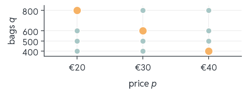
- Prices \(\times\) demand levels: the grid of all (price, bags) pairs
- The roastery’s weekly bags: \((-\infty, 500] \cap [0, \infty) = [0, 500]\); a \(600\)-bag contract makes it \(\emptyset\)
- Today: a function picks dots from that grid: graphs live in \(\mathbb{R}^2\)
Common Issues in the Homework
- Element vs subset: braces build a set: \(\{2\} \subseteq A\) pairs with \(\subseteq\), while \(2 \in A\) pairs with \(\in\); mixing them was the most frequent slip
- Complements reverse inclusion: from \(A \subseteq B\) it follows that \(B^c \subseteq A^c\): writing \(A^c \subseteq B^c\) is the classic denying-the-premise error
- Mixed \(\cup\) and \(\cap\): \(A \cap B \cup C\) is ambiguous: grouping changes the set, so always add parentheses
Which tasks gave you trouble? Bring them up now: we take the time to go through them before we move on to today’s topic.
Warm-Up: Prices and Demands
NoteQuestion
Let \(A = \{20, 30, 40\}\) (prices in €) and \(B = \{400, 500, 600, 800\}\) (bags per week). How many ordered pairs does \(A \times B\) contain? Is \((600, 30)\) one of them?
- \(|A \times B| = |A| \cdot |B| = 3 \cdot 4 = 12\)
- \((600, 30) \notin A \times B\): the first entry must come from \(A\), so \((30, 600)\) is the pair
- Today a price list picks some of these 12 pairs: that choice is a function
Today’s Plan
Session 1 asked which price earns the roastery the most profit. Today: describe price, bags, cost and profit as functions, then read the answer off their shapes.
- What is a function? One price in, one weekly demand out
- Function gallery: shapes of demand, cost, revenue and growth
- Domain in practice: prices the formula and the business allow
- Combining functions: price → bags → cost, and back again
- Reading the shape: floors, ceilings, bends and the best price
Functions as Mappings
One Price, a Chain of Consequences
Session 1's roastery sells its coffee in 1 kg bags. It controls one number: the price \(p\) per bag.
- Price decides weekly demand: €30 sells \(600\) bags, €40 only \(400\)
- Demand decides revenue (\(30 \cdot 600 =\) €18,000) and roasting cost (€200 fixed plus €5 per bag)
- Revenue minus cost decides profit
- Every arrow in \(p \to \text{bags} \to \text{revenue, cost} \to \text{profit}\) is a function
NoteQuestion
Session 1 asked: which price earns the most profit? By the end of today, we can answer.
Which Table Can Quote?
NoteQuestion
The roastery keeps two tables. Which gives exactly one answer for each entry on the left?
Price list
| Price \(p\) (€) | Demand \(q\) (bags) |
|---|---|
| 20 | 800 |
| 30 | 600 |
| 40 | 400 |
Order log
| Customer | Order (bags) |
|---|---|
| Meier | 12 |
| Meier | 30 |
| Kaya | 12 |
The price list: each price gives exactly one demand. Meier gives two different values, so the log has no single answer for Meier.
Exactly One Output per Input
A function is a rule that gives each input exactly one output: the grid lights exactly one dot per column.
WarningCommon Mistake
“Exactly one” restricts the outputs per input: two different inputs may well share the same output.
Function Notation
The price list follows one rule: every €1 more loses 20 bags, so
\[D: \mathbb{R} \to \mathbb{R}, \quad p \mapsto 1200 - 20p\]
- \(D\) is the function’s name; \(p\) is the input
- \(D(p)\) is the output: read “\(D\) of \(p\)”; here \(D(p) = 1200 - 20p\), so \(D(30) = 600\), matching the price list
- \(p \mapsto D(p)\) reads “\(p\) maps to \(D(p)\)”: note the arrow’s little bar
- \(D: A \to B\) names the two sets: inputs from \(A\), outputs in \(B\)
\(D\) and \(D(p)\) are different things: \(D\) is the rule, \(D(p)\) is a number: the value at \(p\).
The Vertical Line Test
The graph of \(D\) on the grid is its set of lit dots. Look at the dashed lines: one lit dot, two circle points.
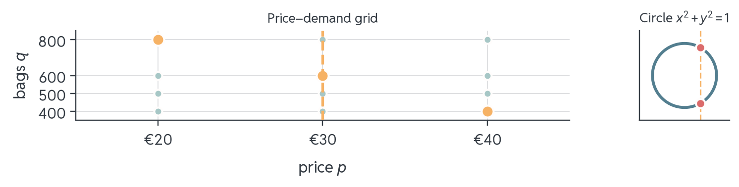
A curve is a function graph \(\Leftrightarrow\) every vertical line hits it at most once: one column, one lit dot.
Your Turn: Function or Not?

NoteQuestion
Which of the two graphs shows \(y\) as a function of \(x\)?
Only Graph B: A fails the vertical line test: \(x = 1\) gives both \(y = 1\) and \(y = -1\). The kink in B is fine.
Domain, Codomain, Range
On the grid, four rows are marked, but row \(500\) is never hit.
For \(D: A \to B\), three sets matter:
- Domain \(A\): all allowed inputs, the graph’s shadow on the horizontal axis
- Codomain \(B\): where outputs are declared to land, here four rows
- Range \(D(A) = \{D(p) : p \in A\}\): collect every output that actually occurs, the graph’s shadow on the vertical axis, here \(\{400, 600, 800\}\)
- Always \(D(A) \subseteq B\): the range is a subset of the codomain
Your Turn: What Is the Range?
NoteQuestion
\(f: \mathbb{R} \to \mathbb{R}\), \(f(x) = x^2 + 1\). Which set is the range of \(f\)?
| (a) \(\mathbb{R}\) | (b) \([0, \infty)\) |
| (c) \([1, \infty)\) | (d) \((1, \infty)\) |
(c): \(x^2 \geq 0\), so \(x^2 + 1 \geq 1\), and the value \(1\) is reached at \(x = 0\): square bracket.
(a) is the codomain, not the range: the declared landing zone is larger than the outputs that actually occur.
Evaluating a Function
To evaluate, substitute the input everywhere the variable appears, just as \(D(30) = 1200 - 20 \cdot 30 = 600\) on the price–demand grid. Take \(f(x) = x^2 - 2x\):
- \(f(3) = 3^2 - 2 \cdot 3 = 9 - 6 = 3\)
- \(f(0) = 0 - 0 = 0\)
- \(f(-1) = (-1)^2 - 2 \cdot (-1) = 1 + 2 = 3\)
- Note: \(f(3) = f(-1) = 3\): two inputs, same output, allowed
Put negative inputs in parentheses before squaring: \((-1)^2 = 1\), not \(-1\).
Plugging in Whole Expressions
“How much does \(f\) change when the input moves from \(a\) to \(a + h\)?”: to answer, substitute the whole expression, in parentheses. Again \(f(x) = x^2 - 2x\):
\[ \begin{aligned} f(a + h) &= (a + h)^2 - 2(a + h) \\ &= (a+h)(a+h) - 2(a+h) = a^2 + 2ah + h^2 - 2a - 2h \end{aligned} \]
WarningCommon Mistake
\(f(a + h) \neq f(a) + f(h)\), check: \(f(1 + 1) = f(2) = 0\), but \(f(1) + f(1) = -1 - 1 = -2\).
Your Turn: Evaluate
NoteQuestion
Again \(f(x) = x^2 - 2x\). What is \(f(-2)\)? Type the number.
\[f(-2) = (-2)^2 - 2 \cdot (-2) = 4 + 4 = 8\]
WarningCommon Mistake
\(f(-2) = 0\) comes from dropping a sign: either \((-2)^2 = -4\) or \(-2 \cdot (-2) = -4\). Both minus signs matter.
Function Gallery
Fixed Costs Plus a Rate
Look where the line starts and how far the dashed step climbs.
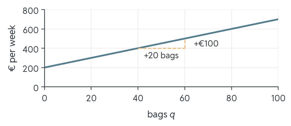
- \(C(q) = 200 + 5q\): intercept \(200\), the fixed cost; slope \(100/20 = 5\) per bag
Your Turn: Slope from Two Points
NoteQuestion
A linear cost function gives \(C(10) = 250\) and \(C(30) = 350\). What are the slope \(m\) and the intercept \(b\)? Type both numbers.
Hint: slope = change in cost ÷ change in bags.
- Slope: \(m = \frac{350 - 250}{30 - 10} = \frac{100}{20} = 5\), €5 per bag; intercept \(b = C(10) - 5 \cdot 10 = 200\), the fixed cost
- So \(C(q) = 200 + 5q\), recovered from two data points
- In general a line \(f(x) = mx + b\) has \(m = \frac{f(x_2) - f(x_1)}{x_2 - x_1}\) everywhere: Session 4 calls this ratio the difference quotient
Price Up, Bags Down
Demand \(D(p) = 1200 - 20p\): each extra euro loses 20 bags (slope \(-20\)). Revenue = price × bags sold: \(R(p) = p \cdot (1200 - 20p)\)
| \(p\) | 0 | 10 | 20 | 30 | 40 | 50 | 60 |
|---|---|---|---|---|---|---|---|
| \(D(p)\) | 1200 | 1000 | 800 | 600 | 400 | 200 | 0 |
| \(R(p)\) | 0 | 10,000 | 16,000 | 18,000 | 16,000 | 10,000 | 0 |
Two forces pull against each other: revenue rises, peaks, falls, symmetrically around \(p = 30\).
Quadratic Functions
Look at the axis of symmetry: the peak sits halfway between the zeros.
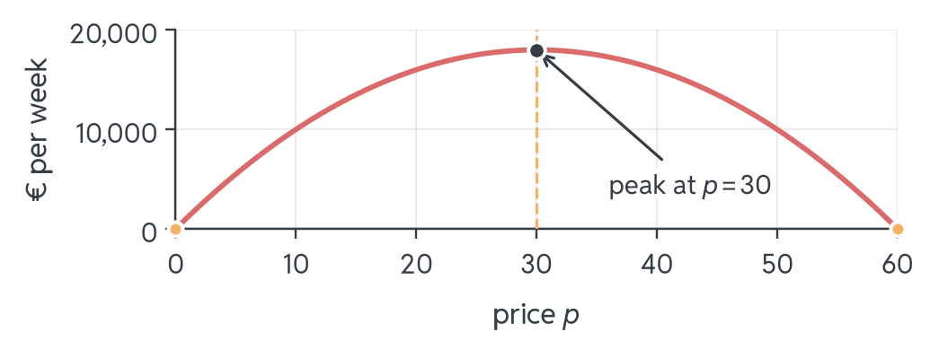
\(R(p) = -20p^2 + 1200p\): a line times a line gives a parabola. Any \(f(x) = ax^2 + bx + c\) opens up if \(a > 0\), down if \(a < 0\); its vertex sits at \(x = -b/(2a)\), here \(-1200/(2 \cdot (-20)) = 30\).
Your Turn: Where Is the Vertex?
NoteQuestion
Another product has revenue \(R(p) = 800p - 10p^2\). Does the parabola open upward or downward, and at which price is the vertex? Type the number.
- \(R(p) = p(800 - 10p)\) is zero at \(p = 0\) and \(p = 80\): peak halfway, at \(p = 40\)
- Formula check: \(-b/(2a) = -800/(2 \cdot (-10)) = 40\) ✓, and \(a = -10 < 0\) means the parabola opens downward
Polynomials: Costs That Bend
Is €5 per bag realistic at any volume? Look at this cost curve’s slope: it flattens, then steepens again.
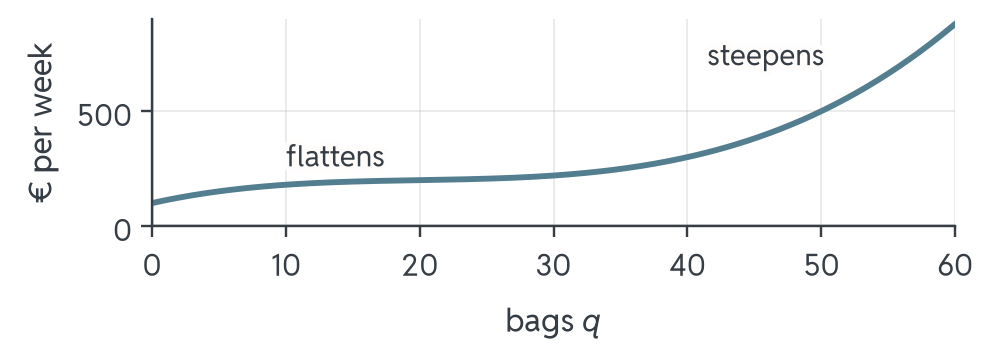
A polynomial \(a_n x^n + \dots + a_0\) of degree \(n\) has up to \(n - 1\) turning points (where the curve turns from rising to falling, or back); this cubic has none but switches from flattening to steepening.
What Does One Bag Cost?
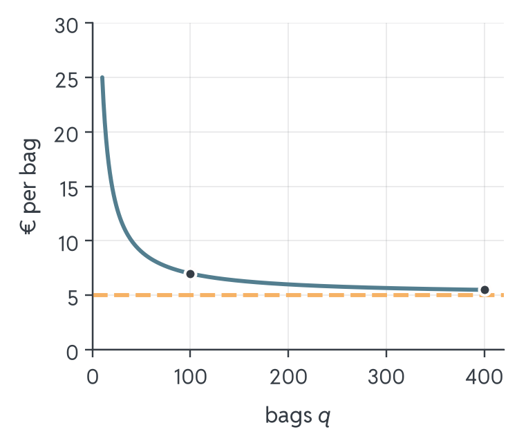
Look at the curve: it explodes near zero, then settles towards €5.
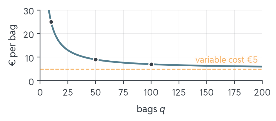
Average cost \(A(q) = C(q)/q = 200/q + 5\): the fixed €200 is spread thinner with every bag: economies of scale.
Rational Functions and \(1/x\)
Look at both branches: they blow up near zero and flatten far out.
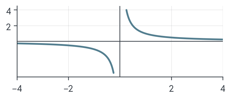
A rational function is a quotient of polynomials. \(A(q)\) is the hyperbola \(1/x\) stretched by \(200\) and lifted by \(5\): a vertical asymptote at \(q = 0\), where it is undefined, and a horizontal asymptote at \(5\).
Below €6 per Bag?
NoteQuestion
Average cost is \(A(q) = \dfrac{200}{q} + 5\). Beyond how many bags does one bag cost less than €6 on average?
- \(\dfrac{200}{q} + 5 < 6 \;\Leftrightarrow\; \dfrac{200}{q} < 1 \;\Leftrightarrow\; q > 200\) (for \(q > 0\))
- And €5 itself? Never: \(\dfrac{200}{q} > 0\) for every \(q > 0\), so the horizontal asymptote is a floor the curve never touches
Compound Interest
Now the input is time: Session 1's €1000 reserve at 5% per year.
| Year \(t\) | 0 | 1 | 2 | 3 | \(t\) |
|---|---|---|---|---|---|
| Compound \(\times 1.05\) | 1000 | 1050 | 1102.50 | 1157.63 | \(1000 \cdot 1.05^t\) |
| Simple \(+\,50\) | 1000 | 1050 | 1100.00 | 1150.00 | \(1000 + 50t\) |
- Interest earns interest: Session 1's product notation \(\prod\), repeated multiplication becomes a power, \(K(t) = K_0 (1 + r)^t\)
- After 15 years: \(1000 \cdot 1.05^{15} \approx\) €2079, so the €1000 doubled somewhere before. When exactly?
Growth and Decay
Any start \(a > 0\), any factor \(b > 0\): \(f(x) = a \cdot b^x\) is an exponential function. \(b > 1\) multiplies by more than 1 (growth); \(0 < b < 1\) keeps only a fraction (decay).
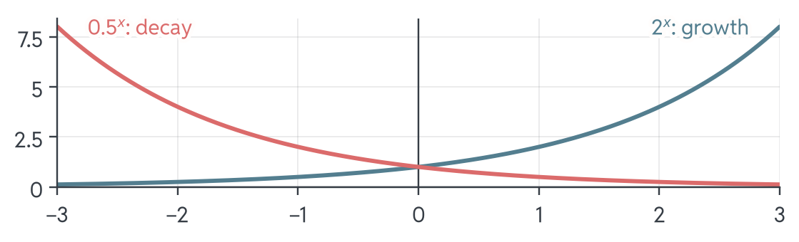
Both pass through \((0,1)\) since \(a = f(0) = 1\); the values stay strictly positive.
Your Turn: Growth or Decay?
NoteQuestion
The resale value of the roastery’s delivery van follows \(V(t) = 50{,}000 \cdot 0.8^t\) (in €, after \(t\) years). Which statement is true?
| (a) The value grows by \(20\%\) per year | (b) The value shrinks by \(20\%\) per year |
| (c) The value shrinks by €10,000 per year | (d) The value reaches €0 after \(5\) years |
(b): base \(0.8 < 1\) means decay, and each year keeps \(80\%\) of the previous value.
WarningCommon Mistake
(c) is the first year only: \(50{,}000 \to 40{,}000\). The second year loses \(8000\), the third \(6400\). And (d) never happens: an exponential stays strictly positive.
Interest Every Second?
NoteQuestion
A bank pays 100% interest per year on €1. Credited once: €2. Credited as two halves of 50%: \(1.5^2 =\) €2.25. What do you hold after one year if interest is credited every second?
| (a) €2.25 | (b) about €2.72 |
| (c) about €10 | (d) unlimited, it keeps growing |
| Credited | yearly | monthly | daily | every second |
|---|---|---|---|---|
| After 1 year | €2 | €2.61 | €2.71 | €2.71828… |
- (b): crediting more often approaches Euler’s number \(e \approx 2.71828\)
Continuous Growth
Credited \(n\) times a year at rate \(r\): \(\left(1 + \frac{r}{n}\right)^n \to e^r\) per year as \(n \to \infty\); over \(t\) years, \((e^r)^t = e^{rt}\), giving \(K(t) = K_0 \, e^{rt}\): continuous growth
Logarithms: Undoing \(e^x\)
Back to the €1000: which \(t\) gives \(1.05^t = 2\)? Trying \(t = 14\) (\(1.98\)) and \(t = 15\) (\(2.08\)) only brackets it. We need an operation that returns the exponent.
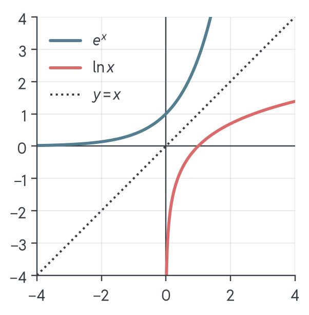
The natural logarithm \(\ln x\) answers: which power of \(e\) gives \(x\)?
\[y = \ln x \;\, \Leftrightarrow \;\, x = e^y\]
\(\ln\) also cracks \(1.05^t = 2\): taking \(\ln\) of both sides brings \(t\) down from the exponent (see Solving for the Exponent).
Reading \(\ln x\)
- Input and output swap roles: the graph is \(e^x\) mirrored across \(y = x\)
- Only \(x > 0\): no power of \(e\) is zero or negative
- \(\ln 1 = 0\), \(\ln e = 1\), and \(\ln x < 0\) for \(0 < x < 1\)
Log Rules Are Exponent Rules
Count doublings: top = exponent, bottom = growth factor \(2^x\).
| \(x\) | \(-1\) | \(0\) | \(1\) | \(2\) | \(3\) | \(4\) | \(5\) | \(6\) | \(7\) | \(8\) |
|---|---|---|---|---|---|---|---|---|---|---|
| \(2^x\) | \(\frac12\) | \(1\) | \(2\) | \(4\) | \(8\) | \(16\) | \(32\) | \(64\) | \(128\) | \(256\) |
- \(8 \cdot 32 = 256\) while \(3 + 5 = 8\): multiplying factors adds exponents, \(a^x a^y = a^{x+y}\)
- \(256 / 32 = 8\) while \(8 - 5 = 3\): dividing subtracts, \(a^x / a^y = a^{x-y}\)
- \(8^2 = 64\) while \(2 \cdot 3 = 6\): repeating multiplies, \((a^x)^k = a^{kx}\)
Halvings and Half-Doublings
| \(x\) | \(-1\) | \(0\) | \(1\) | \(2\) | \(3\) | \(4\) | \(5\) | \(6\) | \(7\) | \(8\) |
|---|---|---|---|---|---|---|---|---|---|---|
| \(2^x\) | \(\frac12\) | \(1\) | \(2\) | \(4\) | \(8\) | \(16\) | \(32\) | \(64\) | \(128\) | \(256\) |
- One step left: no doubling is the factor \(1\), one halving is \(2^{-1} = \frac12\)
- One step further: two half-doublings make one doubling, so \(2^{1/2} = \sqrt{2}\)
Rules for Logarithms
\(\ln\) reads the table upwards in base \(e\): it returns the exponent, so the exponent rules become
\[\ln(xy) = \ln x + \ln y \qquad \ln\frac{x}{y} = \ln x - \ln y \qquad \ln(x^k) = k \ln x\]
The power rule pulls an unknown down from the exponent: that is how logs answer “how long until…?”
WarningCommon Mistake
\(\ln(x + y) \neq \ln x + \ln y\): there is no row in the table for adding factors. The rules work for products, not sums.
Your Turn: Which Log Rule?
NoteQuestion
Which expression equals \(\ln(x^2 y)\) for \(x, y > 0\)?
| (a) \(2 \ln x + \ln y\) | (b) \(2 \ln x \cdot \ln y\) |
| (c) \(\ln(x^2) \cdot \ln y\) | (d) \(2\,(\ln x + \ln y)\) |
(a): the product rule splits \(\ln(x^2 y) = \ln(x^2) + \ln y\), then the power rule gives \(\ln(x^2) = 2 \ln x\).
(d) would be \(\ln(x^2 y^2)\): the factor \(2\) belongs to \(x\) only, so apply the power rule after splitting the product.
Solving for the Exponent
The €1000 again: when is \(1000 \cdot 1.05^t = 2000\)?
- Isolate the power: \(1.05^t = 2\)
- Take \(\ln\) and pull \(t\) down: \(t \ln 1.05 = \ln 2\)
- Divide: \(t = \dfrac{\ln 2}{\ln 1.05} \approx \dfrac{0.6931}{0.0488} \approx 14.2\) years, inside the bracket 14 to 15 we guessed
Isolate, take \(\ln\), divide: every “how long until” question. For decay (\(0 < b < 1\)) the divisor \(\ln b\) is negative, so an inequality flips.
Your Turn: When Has It Doubled?
NoteQuestion
Capital grows continuously at \(r = 5\%\): \(K(t) = K_0 \cdot e^{0.05t}\). When has it doubled?
| (a) 10 years | (b) about 13.9 years |
| (c) 20 years | (d) depends on \(K_0\) |
\[e^{rt} = 2 \quad \Rightarrow \quad rt = \ln 2 \quad \Rightarrow \quad t = \frac{\ln 2}{r} \approx \frac{0.693}{0.05} \approx 13.9\]
- (b): \(K_0\) cancels, (d) fails: €10 and €10 million double equally fast
- Rule of 70: doubling time \(\approx 70 \,/\, (\text{rate in } \%)\); yearly crediting (14.2 years) is slightly slower
Domain in Practice
Where Does the Formula Break?
NoteQuestion
Type into your calculator: average cost \(A(q) = 200/q + 5\) at \(q = 0\), \(\sqrt{x}\) at \(x = -4\), \(\ln x\) at \(x = 0\). What happens?
Three error messages, and they are the three red flags:
- Division by zero: denominators must stay \(\neq 0\)
- Even roots of negatives: under \(\sqrt{\phantom{x}}\) we need \(\geq 0\)
- Logs of non-positives: inside \(\ln\) we need \(> 0\) (strictly!)
With no domain stated, take the maximal domain: every real input that triggers no error. Polynomials and exponentials never do.
Finding the Domain: Examples
| Function | Restriction | Maximal domain |
|---|---|---|
| \(\dfrac{1}{x - 3}\) | \(x - 3 \neq 0\) | \(\mathbb{R} \setminus \{3\}\) |
| \(\sqrt{2x + 6}\) | \(2x + 6 \geq 0\) | \([-3, \infty)\) |
| \(\ln(5 - x)\) | \(5 - x > 0\) | \((-\infty, 5)\) |
The results are intervals. Session 1's notation pays off: square bracket at \(-3\) (\(\sqrt{0}\) is fine), round bracket at \(5\) (\(\ln 0\) is not).
Your Turn: Find the Domain
NoteQuestion
What is the maximal domain of \(f(x) = \dfrac{\sqrt{x - 2}}{x - 4}\)?
- The root needs \(x - 2 \geq 0\), so \(x \geq 2\)
- The denominator needs \(x - 4 \neq 0\), so \(x \neq 4\)
- Both must hold, intersect the conditions: \([2, 4) \cup (4, \infty)\)
Collect every restriction first, then combine: one forgotten condition is the typical exam slip.
Domains in Business
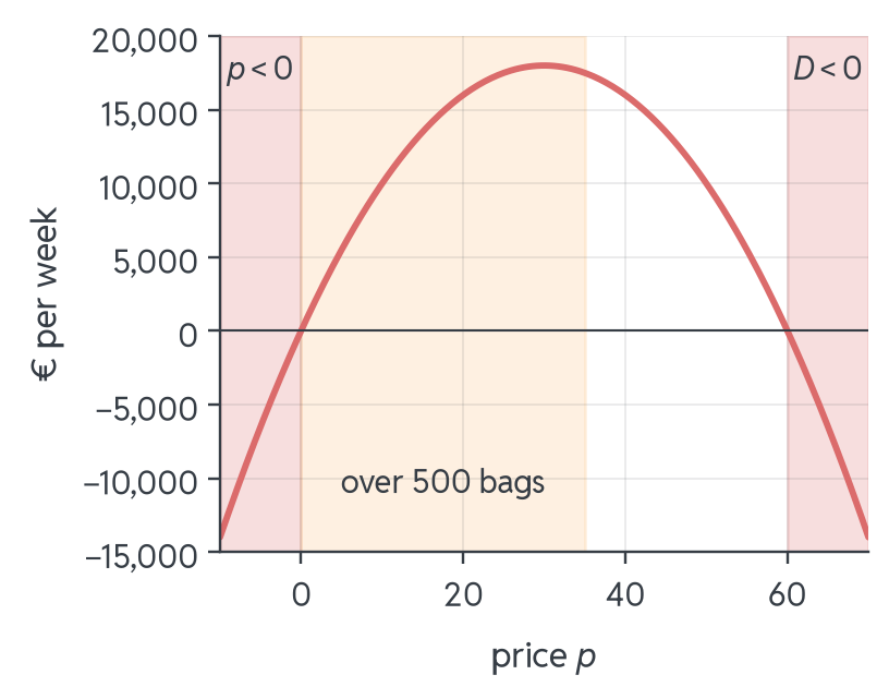
Look at the shaded parts: the formula keeps going, the business does not.
- \(p \geq 0\) and \(D(p) \geq 0\) force \(p \in [0, 60]\)
- Capacity caps bags at 500: \(1200 - 20p \leq 500\), so \(700 \leq 20p\), so \(p \geq 35\), a floor on the price
- The model domain is \([0, 60] \cap [35, \infty) = [35, 60]\): an intersection, as in Session 2
Combining Functions
A Checkout in Two Steps
The roastery’s webshop applies a €10 voucher \(v(p) = p - 10\) and 19% VAT \(T(p) = 1.19p\) to a €50 basket.
NoteQuestion
What does the customer pay? Shout your number.
\[50 \xrightarrow{\;v\;} 40 \xrightarrow{\;T\;} 47.60 \qquad\qquad 50 \xrightarrow{\;T\;} 59.50 \xrightarrow{\;v\;} 49.50\]
Same two machines, different order, different bill.
WarningCommon Mistake
Assuming the order can be swapped: it rarely can. Always check which function acts first.
Composition: Machines in a Row
Feeding one function’s output into the next is a composition. The roastery’s cost depends on bags, and bags depend on price: chain \(D\), then \(C\):
\[(C \circ D)(p) = C(D(p)) = 200 + 5(1200 - 20p) = 6200 - 100p\]
- The function next to \(p\) acts first, inside out: \(D\) then \(C\)
- Same for the checkout: voucher first \((T \circ v)(p)\), tax first \((v \circ T)(p)\): not interchangeable
- The second machine must accept the first’s output: \(\sqrt{x - 5}\) needs \(x \geq 5\)
Your Turn: Where Will Profit Peak?
NoteQuestion
Profit as a function of price is \(\pi(p) = R(p) - C(D(p))\). Revenue peaks at €30. The profit-maximising price is…
| (a) below €30 | (b) exactly €30 |
| (c) above €30 | (d) impossible to tell |
\[\pi(p) = (1200p - 20p^2) - (6200 - 100p) = -20p^2 + 1300p - 6200\]
(c): the vertex sits at \(p = -\dfrac{1300}{2 \cdot (-20)} = 32.5\). A higher price sells fewer bags, and fewer bags cost less to roast, so the peak moves right of the revenue peak.
Running the Machine Backwards
NoteQuestion
A customer paid €47.60 after voucher and VAT. What was the basket?
- Undo the last step first: \(47.60 / 1.19 = 40\), then undo the voucher: \(40 + 10 = 50\)
- Running the machine backwards gives the inverse \(f^{-1}\): \(f(a) = b \;\Leftrightarrow\; f^{-1}(b) = a\)
- Here \(f = T \circ v\): \(f(50) = 47.60\) and \(f^{-1}(47.60) = 50\), the same pair read the other way
Finding an Inverse
Swap-and-solve: the output becomes the given, the input the unknown. Write \(y = f(x)\) and solve for \(x\).
Demand example: \(q = D(p) = 1200 - 20p\):
\[q = 1200 - 20p \quad \Rightarrow \quad 20p = 1200 - q \quad \Rightarrow \quad p = 60 - \frac{q}{20}\]
- \(D^{-1}(q) = 60 - \frac{q}{20}\): the price needed to sell exactly \(q\) bags
- Check with a pair: \(D(30) = 600\) and \(D^{-1}(600) = 60 - 30 = 30\) ✓
- \(D\) multiplies by \(-20\) then adds \(1200\); \(D^{-1}\) undoes it in reverse: the checkout rule again
Does More Always Mean More?
Higher price, more revenue? Look at \(R(p)\):
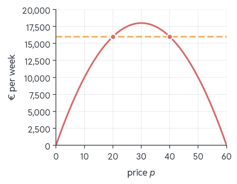
\(f\) is strictly increasing on an interval if \(x_1 < x_2 \Rightarrow f(x_1) < f(x_2)\). \(R\) is strictly increasing on \([0, 30]\) and strictly decreasing on \([30, 60]\).
The dashed line marks €16,000. Which price earned it?
When Backwards Fails
\(R(20) = R(40) = 16{,}000\): which price earned €16,000? No unique answer, so \(R\) has no inverse on \([0, 60]\).
An inverse needs \(f\) one-to-one: each output from exactly one input. Horizontal line test: every horizontal line hits the graph at most once.
Strictly monotone \(\Rightarrow\) one-to-one: on \([0, 30]\) \(R\) has an inverse, just as \(x^2\) on \([0, \infty)\) has \(\sqrt{x}\).
Your Turn: Undo the Function
NoteQuestion
Let \(f(x) = 3x - 6\). What is \(f^{-1}(9)\)?
| (a) \(9\) | (b) \(5\) |
| (c) \(21\) | (d) \(\frac{1}{21}\) |
(b): undo in reverse order: \(9 + 6 = 15\), then \(15 / 3 = 5\). Check: \(f(5) = 9\) ✓
WarningCommon Mistake
(a) undoes in the wrong order (\(9/3 + 6\)), (c) runs \(f\) forwards, and (d) reads \(f^{-1}\) as \(\frac{1}{f}\): for functions, the exponent \(-1\) means undo, not divide.
The Mirror Property
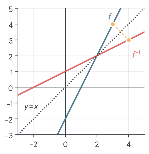
Look at the dashed segment: it flips across the dotted line \(y = x\).
For \(f(x) = 2x - 2\), \(f(3) = 4\) becomes \(f^{-1}(4) = 3\): swapping coordinates reflects the graph across \(y = x\). That is why \(\ln x\) mirrors \(e^x\).
Your Turn: Invertible or Not?
NoteQuestion
Which of these functions is not one-to-one on \(\mathbb{R}\), and therefore has no inverse there?
| (a) \(f(x) = 2x + 1\) | (b) \(f(x) = e^x\) |
| (c) \(f(x) = x^2 - 4\) | (d) \(f(x) = x^3\) |
(c): \(f(2) = f(-2) = 0\), one output from two inputs, so it fails the horizontal line test.
The other three are strictly increasing on all of \(\mathbb{R}\): each output is hit once, so each has an inverse. Same story as \(D(p) = 1200 - 20p\), which is strictly decreasing and has \(D^{-1}\), while \(R(p)\) earns €16,000 at two prices and has none.
Reading the Shape
Is There a Floor or a Ceiling?
\(A(q) = 200/q + 5\) settles towards the dashed floor but never touches it.
- Bounded below: some \(m\) has \(f(x) \geq m\) for all \(x\); for \(A(q)\), \(m = 5\), never reached (€7 at 100, €5.50 at 400)
- Bounded above: some \(M\) has \(f(x) \leq M\) for all \(x\); revenue’s \(18{,}000\) is reached, at \(p = 30\)
Does Each Extra Euro Add Less?
The roastery’s extra bags from an advertising budget \(a\) (in €1000): \(S(a) = 100\sqrt{a}\). Compare with the €1000 reserve at 5% from earlier.
| Step | \(0 \to 1\) | \(1 \to 2\) | \(2 \to 3\) | \(3 \to 4\) |
|---|---|---|---|---|
| Extra bags from the next €1000 | \(+100\) | \(+41\) | \(+32\) | \(+27\) |
| Extra interest in the next year | €50.00 | €52.50 | €55.13 | €57.88 |
Bag gains shrink: diminishing returns. Interest gains grow. Both curves rise, but they bend in opposite directions.
Convex or Concave?
Look at the dashed chords: left, above the curve; right, below it.

- Convex: every chord lies on or above the graph: gains grow
- Concave: every chord lies on or below the graph: diminishing returns
- This is the chord test; Sessions 4–5 turn it into a calculation
Your Turn: How Does It Bend?
NoteQuestion
The van’s resale value \(V(t) = 50{,}000 \cdot 0.8^t\) loses €10,000, then €8000, then €6400 per year. Which describes the graph?
| (a) Decreasing and concave | (b) Decreasing and convex |
| (c) Increasing and convex | (d) Decreasing, neither shape |
(b): the losses shrink, so the curve falls ever more gently and bends upward. Every chord lies on or above the graph.
Convex says nothing about rising: the direction (monotone) and the bend (convex or concave) are two separate questions.
So Which Price?
Profit \(\pi(p) = -20p^2 + 1300p - 6200\) peaks at €32.50; look at the shaded band, the only prices the roastery can actually charge.
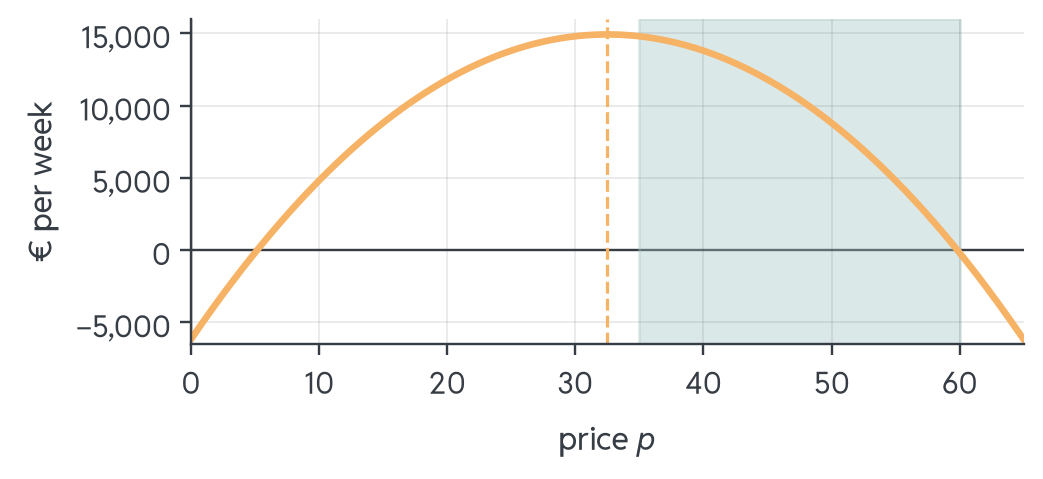
€32.50 lies left of \([35, 60]\): right of its peak \(\pi\) only falls, so the roastery charges €35.
Closing
Key Takeaways
- Function: each price gives exactly one demand, \(D(p) = 1200 - 20p\)
- Gallery: linear demand and cost, a revenue parabola, rational average cost; \(\ln\) finds when savings double
- Domain: \(D(p) \geq 0\) and the capacity of 500 bags leave prices in \([35, 60]\)
Key Takeaways: Chains & Shape
- Composition: cost as a function of price is \(C(D(p))\), with \(D\) first; profit is \(\pi(p) = R(p) - C(D(p))\)
- Inverse: \(D\) is strictly decreasing, so \(D^{-1}(q) = 60 - q/20\) exists: the price for a target volume
- Shape: \(\pi\) is a concave parabola peaking at €32.50 and falling on \([35, 60]\): the roastery charges €35
Until the Next Session
- Work through the Tasks: problems with worked solutions
- Check yourself with the Self-Test quiz
- Keep the Cheatsheet next to you while practising
- Note down anything unclear: we start next session with your questions
When a function confuses you, sketch it: five plotted points reveal more than ten minutes of staring at the formula.
Preview: Session 04: Differentiation
- Central question: how fast does a function change?
- On today’s \(R(p)\): what does a €1 price rise add at \(p = 10\), and at \(p = 30\)? Take a guess
- Today’s \(f(a + h)\) becomes the difference quotient; the tangent gives the slope of a curve
- Marginal cost and marginal revenue: the language of decisions
- Today’s chord test becomes a quick sign check, and \(e^x\) reveals its superpower
See you there, and bring your questions!
Literature & Further Reading
- These sessions cover the essentials: textbooks offer more depth and practice
- Start with Sydsæter et al. (2012) or Jacques (2015); full recommendations on the tutorial’s literature page
Jacques, Ian. 2015. Mathematics for Economics and Business. 8th ed. Always Learning. Pearson.
Sydsæter, Knut, Peter J. Hammond, and Arne Strøm. 2012. Essential Mathematics for Economic Analysis. 4th ed. Pearson.