Session 03 - Functions

Mathematics for Master Students

Dr. Tobias Vlcek

Recap & Your Questions

Session 02 in a Nutshell

A set is an unordered collection of distinct elements: \(\in\) for elements, \(\subseteq\) for sets
\(\cup\), \(\cap\), \(\setminus\), \(^c\) mirror or, and, not: De Morgan flips \(\cup\) and \(\cap\)
Counting a union: \(|A \cup B| = |A| + |B| - |A \cap B|\)
\(A \times B\) collects ordered pairs: \(\mathbb{R} \times \mathbb{R} = \mathbb{R}^2\) is the plane
Constraints are sets, and they combine by intersection
Today: functions map between sets, and their graphs live in \(\mathbb{R}^2\)

Common Issues in the Homework

Element vs subset: braces build a set: \(\{2\} \subseteq A\) pairs with \(\subseteq\), while \(2 \in A\) pairs with \(\in\); mixing them was the most frequent slip
Complements reverse inclusion: from \(A \subseteq B\) it follows that \(B^c \subseteq A^c\): writing \(A^c \subseteq B^c\) is the classic inversion error
Mixed \(\cup\) and \(\cap\): \(A \cap B \cup C\) is ambiguous: grouping changes the set, so always add parentheses

Which tasks gave you trouble? Bring them up now: we take the time to go through them before we move on to today’s topic.

Warm-Up: One Quick Evaluation

Question

Let \(A = \{1, 2, 3, 4\}\) and \(B = \{3, 4, 5\}\). Compute \(\;(A \cup B) \setminus (A \cap B)\).

Inside out: \(A \cup B = \{1, 2, 3, 4, 5\}\) and \(A \cap B = \{3, 4\}\)
Removing the intersection: \((A \cup B) \setminus (A \cap B) = \{1, 2, 5\}\)
In words: everything in exactly one of the two sets: “either, but not both”

Today’s Plan

What is a function?: exactly one output for every input
Function gallery: linear, quadratic, polynomial, rational, exponential, logarithm
Domain in practice: which inputs are allowed
Combining functions: composition and inverses
Properties: monotone, bounded, convex vs concave

Functions as Mappings

What Is a Function?

A function \(f: A \to B\) is a rule that assigns to each element \(x \in A\) exactly one element \(f(x) \in B\).

It maps between two sets: the ones from last session
Think of a machine: input \(x\) goes in, output \(f(x)\) comes out
“Exactly one” makes it predictable: same input, same output, every time

Common Mistake

“Exactly one” restricts the outputs per input. Two different inputs may share the same output: that is perfectly fine.

Function Notation

\[f: \mathbb{R} \to \mathbb{R}, \quad x \mapsto 2x + 5\]

\(f\) is the function’s name; \(x\) is the input, also called the argument
\(f(x)\) is the output: read “\(f\) of \(x\)”; here \(f(x) = 2x + 5\)
\(x \mapsto f(x)\) reads “\(x\) maps to \(f(x)\)”: note the little bar on the arrow
\(f: A \to B\) names the two sets: inputs come from \(A\), outputs land in \(B\)

\(f\) and \(f(x)\) are different things: \(f\) is the rule, \(f(x)\) is a number: the value at \(x\).

Domain, Codomain, Range

For \(f: A \to B\), three sets matter:

The domain \(A\): all allowed inputs
The codomain \(B\): where outputs are declared to land
The range \(f(A) = \{f(x) : x \in A\}\): the outputs that actually occur
Always \(f(A) \subseteq B\): the range is a subset of the codomain

Example: \(f: \mathbb{R} \to \mathbb{R}\), \(f(x) = x^2\): codomain \(\mathbb{R}\), but range \([0, \infty)\): no square is negative.

Evaluating a Function

To evaluate, substitute the input everywhere the variable appears, take \(f(x) = x^2 - 2x\):

\(f(3) = 3^2 - 2 \cdot 3 = 9 - 6 = 3\)
\(f(0) = 0 - 0 = 0\)
\(f(-1) = (-1)^2 - 2 \cdot (-1) = 1 + 2 = 3\)
Note: \(f(3) = f(-1) = 3\): two inputs, same output, allowed

Put negative inputs in parentheses before squaring: \((-1)^2 = 1\), not \(-1\).

Plugging in Whole Expressions

The input can be an expression: substitute all of it, in parentheses. Again \(f(x) = x^2 - 2x\):

\[f(a + h) = (a + h)^2 - 2(a + h) = a^2 + 2ah + h^2 - 2a - 2h\]

Common Mistake

\(f(a + h) \neq f(a) + f(h)\), check: \(f(1 + 1) = f(2) = 0\), but \(f(1) + f(1) = -1 - 1 = -2\).

Expressions like \(f(a + h)\) are the raw material of Session 4: “how much does \(f\) change when the input moves by \(h\)?”

The Vertical Line Test

The graph of \(f\) is the set \(\{(x, f(x)) : x \in A\} \subseteq \mathbb{R}^2\): ordered pairs, as in Session 2.

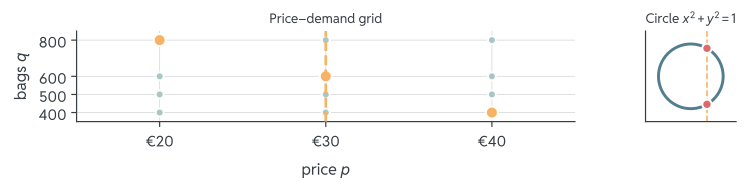
A curve is the graph of a function \(\Leftrightarrow\) every vertical line hits it at most once
Why: one input \(x\) must yield exactly one output
The circle \(x^2 + y^2 = 1\) fails: at \(x = 0\) it contains two points, \(y = 1\) and \(y = -1\)
Lines, parabolas and exponential curves all pass

Your Turn: Which Graph is a Function?

Question

Which of the two graphs shows \(y\) as a function of \(x\)?

Only Graph B: A fails the vertical line test: \(x = 1\) gives both \(y = 1\) and \(y = -1\). The kink in B is fine.

Functions in Business

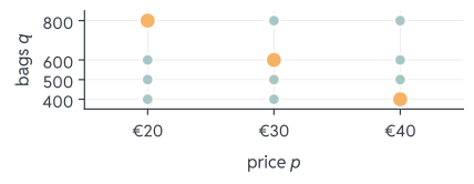
Functions map decisions to outcomes, the core of every quantitative model:

Cost function \(C(q)\): production quantity \(\to\) total cost
Demand function \(D(p)\): price \(\to\) units sold
Production function: input (labor hours) \(\to\) output (units)
One decision in, one predicted outcome out: that is why models must be functions

Whenever a spreadsheet column is computed from another column, there is a function behind it.

Function Gallery

Linear Functions

\[f(x) = mx + b\]

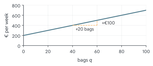
Slope \(m\): the output changes by \(m\) for each unit of input, constant everywhere
Intercept \(b = f(0)\): the starting level
From two points on the graph: \(m = \frac{f(x_2) - f(x_1)}{x_2 - x_1}\)
The workhorse of business models: constant rates

A Linear Cost Function

\(C(x) = 200 + 5x\): the fixed costs are the intercept, the variable cost per unit is the slope.

Quadratic Functions

\[f(x) = ax^2 + bx + c, \quad a \neq 0\]

The graph is a parabola: opens upward if \(a > 0\), downward if \(a < 0\)
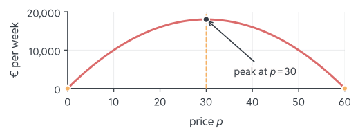
The turning point is the vertex, located at \(x = -\frac{b}{2a}\)
Downward parabolas model trade-offs: revenue rises with price, until demand collapses

A Quadratic Revenue Function

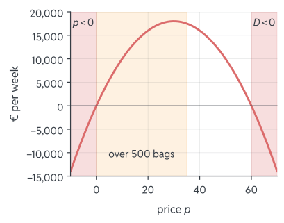
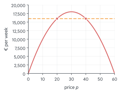
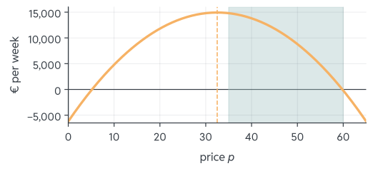
Demand \(D(p) = 1200 - 20p\) gives revenue \(R(p) = p \cdot D(p) = 1200p - 20p^2\): the vertex \(p = -\frac{1200}{2 \cdot (-20)} = 30\) is the revenue-maximal price.

Polynomials

\[f(x) = a_n x^n + \dots + a_1 x + a_0 \qquad \text{degree } n = \text{highest power}\]

Degree \(n\) allows up to \(n\) roots and up to \(n - 1\) turning points: far from the origin the leading term \(a_n x^n\) dominates (\(f(x) = x^3 - 3x\) above behaves like \(x^3\)).

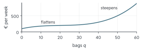
Cubic cost curves \(C(x) = ax^3 + bx^2 + cx + d\) are the classic economics example: costs rise steeply, flatten, then steepen again.

Rational Functions

\[f(x) = \frac{p(x)}{q(x)} \qquad \text{a quotient of two polynomials}\]

Defined only where \(q(x) \neq 0\): division by zero is the first domain trap
Near a zero of the denominator, values explode: a vertical asymptote
For large inputs, the graph can settle toward a horizontal asymptote

The Hyperbola \(f(x) = 1/x\)

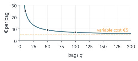
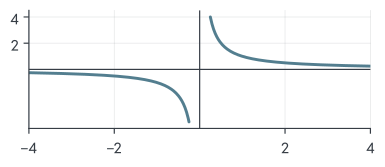
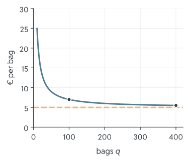
Both axes are asymptotes. Business example: with \(C(x) = 200 + 5x\), the cost per unit is \(\frac{C(x)}{x} = \frac{200}{x} + 5\): it falls toward 5 as volume grows: economies of scale.

Exponential Functions

\[f(x) = a \cdot b^x, \quad b > 0\]

The variable sits in the exponent: each step multiplies by \(b\)
\(b > 1\): growth (interest, booming demand); \(0 < b < 1\): decay (depreciation, churn)
\(a = f(0)\) is the starting value
The standard base is Euler’s number \(e \approx 2.71828\): Sessions 4–5 show why it is so convenient

Growth and Decay

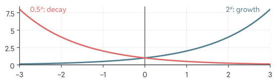
Both stay strictly positive and pass through \((0, 1)\): an exponential never reaches zero.

Compound Interest

Deposit \(K_0\) at annual rate \(r\), each year multiplies the balance by \((1 + r)\):

\[K_t = K_0 \cdot \underbrace{(1+r)(1+r) \dots (1+r)}_{t \text{ factors}} = K_0 \cdot (1+r)^t\]

Session 1’s product idea in action: repeated multiplication becomes a power
€1000 at \(r = 0.05\): after 15 years \(1000 \cdot 1.05^{15} \approx\) €2079: more than doubled
As a function of time \(t\), this is exponential growth with base \(b = 1.05\)

Logarithms: Undoing \(e^x\)

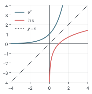
The natural logarithm \(\ln x\) answers: which exponent produces \(x\)?

\[y = \ln x \;\, \Leftrightarrow \;\, x = e^y\]

\(\ln x\) is the mirror image of \(e^x\) across the diagonal
Defined only for \(x > 0\)
\(\ln 1 = 0\) and \(\ln e = 1\)

Rules for Logarithms

\[\ln(xy) = \ln x + \ln y \qquad \ln\frac{x}{y} = \ln x - \ln y \qquad \ln(x^k) = k \ln x\]

Logs turn products into sums and powers into multiples
The power rule pulls the unknown down from the exponent: that is why logs solve growth questions
Other bases reduce to \(\ln\): \(\log_b x = \frac{\ln x}{\ln b}\)

Common Mistake

\(\ln(x + y) \neq \ln x + \ln y\): the rules work for products, not sums.

Your Turn: When Has It Doubled?

Question

With continuous growth at rate \(r\), capital follows \(K_t = K_0 \cdot e^{rt}\). When has it doubled?

\[e^{rt} = 2 \quad \Rightarrow \quad rt = \ln 2 \quad \Rightarrow \quad t = \frac{\ln 2}{r} \approx \frac{0.693}{r}\]

At \(r = 5\%\): \(t \approx \frac{0.693}{0.05} \approx 13.9\) years: independent of the starting amount
The same trick handles yearly compounding: \(1.05^t = 2\) gives \(t = \frac{\ln 2}{\ln 1.05} \approx 14.2\) years

Domain in Practice

The Maximal Domain

If no domain is stated, take the maximal domain: the largest set of reals on which the formula is defined.

Three red flags:

Division by zero: denominators must stay \(\neq 0\)
Even roots of negatives: under \(\sqrt{\phantom{x}}\) we need \(\geq 0\)
Logs of non-positives: inside \(\ln\) we need \(> 0\) (strictly!)

Everything else (polynomials, exponentials) is safe on all of \(\mathbb{R}\).

Finding the Domain: Examples

Function	Restriction	Maximal domain
\(\dfrac{1}{x - 3}\)	\(x - 3 \neq 0\)	\(\mathbb{R} \setminus \{3\}\)
\(\sqrt{2x + 6}\)	\(2x + 6 \geq 0\)	\([-3, \infty)\)
\(\ln(5 - x)\)	\(5 - x > 0\)	\((-\infty, 5)\)

The results are intervals. Session 1’s notation pays off: square bracket at \(-3\) (\(\sqrt{0}\) is fine), round bracket at \(5\) (\(\ln 0\) is not).

Your Turn: Find the Domain

Question

What is the maximal domain of \(\;f(x) = \dfrac{\sqrt{x - 2}}{x - 4}\;\)?

The root needs \(x - 2 \geq 0\), so \(x \geq 2\)
The denominator needs \(x - 4 \neq 0\), so \(x \neq 4\)
Both must hold, intersect the conditions: \([2, 4) \cup (4, \infty)\)

Collect every restriction first, then combine: one forgotten condition is the typical exam slip.

Domains in Business

Business adds its own restrictions on top of the math:

Quantities are non-negative: \(q \in [0, \infty)\): no producing \(-50\) pallets
Capacity caps the allowed quantities: \(q \in [0, 500]\)
Prices must keep demand meaningful: \(D(p) = 1200 - 20p \geq 0\) forces \(p \in [0, 60]\)
Model domain = mathematical domain \(\cap\) business constraints: an intersection, as in Session 2

Combining Functions

Composition of Functions

Chaining two functions, apply \(g\) first, then \(f\) to the result:

\[(f \circ g)(x) = f(g(x))\]

Read from the inside out: the inner function acts first
Example: \(g(x) = 2x\) and \(f(x) = x + 3\): \(\;(f \circ g)(x) = f(2x) = 2x + 3\)
But \((g \circ f)(x) = g(x + 3) = 2x + 6\): not the same
Business reading: multi-stage processes, the output of one stage feeds the next

Order Matters: Voucher and VAT

A webshop applies a €10 voucher \(v(p) = p - 10\) and 19% VAT \(t(p) = 1.19p\) to a net price \(p\):

Voucher first, then tax: \((t \circ v)(p) = 1.19(p - 10) = 1.19p - 11.90\)
Tax first, then voucher: \((v \circ t)(p) = 1.19p - 10\)
The results differ by €1.90 on every order: for the customer, voucher first is cheaper

Common Mistake

Assuming \(f \circ g = g \circ f\): in general, the order cannot be swapped. Always check which function acts first.

Your Turn: Compose in the Right Order

Question

Let \(f(x) = x^2\) and \(g(x) = x + 1\). Compute \(\;(f \circ g)(2)\;\) and \(\;(g \circ f)(2)\).

\((f \circ g)(2) = f(g(2)) = f(3) = 9\)
\((g \circ f)(2) = g(f(2)) = g(4) = 5\)
Inside out, always, and the order visibly changes the answer

Inverse Functions

The inverse \(f^{-1}\) undoes \(f\):

\[f(a) = b \quad \Leftrightarrow \quad f^{-1}(b) = a\]

It exists only if \(f\) is one-to-one: every output comes from exactly one input
Graph check: every horizontal line hits the graph at most once
\(f(x) = x^2\) on \(\mathbb{R}\) fails: \(f(2) = f(-2) = 4\): which input produced \(4\)?
Restricting to \([0, \infty)\) repairs it: there \(f^{-1}(x) = \sqrt{x}\)

Finding an Inverse

Write \(y = f(x)\), solve for \(x\), then read the result as a function of the output.

Demand example: \(q = D(p) = 1200 - 20p\):

\[q = 1200 - 20p \quad \Rightarrow \quad 20p = 1200 - q \quad \Rightarrow \quad p = 60 - \frac{q}{20}\]

\(D^{-1}(q) = 60 - \frac{q}{20}\): the price needed to sell exactly \(q\) units
Check with a pair: \(D(30) = 600\) and \(D^{-1}(600) = 60 - 30 = 30\) ✓
Domain and range swap: the domain of \(D^{-1}\) is the range of \(D\)

The Notation Trap: \(f^{-1} \neq 1/f\)

\(f^{-1}(x)\) is the inverse function: the \(-1\) sits on the function name
The reciprocal of the value is written \((f(x))^{-1} = \frac{1}{f(x)}\)
Example \(f(x) = 2x\): \(\;f^{-1}(x) = \frac{x}{2}\), but \(\frac{1}{f(x)} = \frac{1}{2x}\): completely different

Common Mistake

Reading \(f^{-1}\) as “one over \(f\)”: for functions, the exponent \(-1\) means undo, not divide.

The Mirror Property

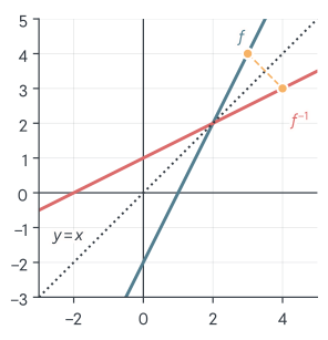
Swapping input and output reflects the graph across \(y = x\): the point \((3, 4)\) on \(f\) becomes \((4, 3)\) on \(f^{-1}\): exactly how \(\ln x\) mirrored \(e^x\).

Properties

Monotonicity

\(f\) is increasing if \(x_1 < x_2 \Rightarrow f(x_1) \leq f(x_2)\): strictly increasing with \(<\). Decreasing works the same way, flipped.

Graph reading: strictly increasing = rises left to right, everywhere
Costs increase in quantity; demand decreases in price
Strictly monotone \(\Rightarrow\) one-to-one \(\Rightarrow\) invertible: that is why \(e^x\) has an inverse but \(x^2\) on \(\mathbb{R}\) does not

Boundedness

\(f\) is bounded above if some \(M\) satisfies \(f(x) \leq M\) for all \(x\): bounded below works with \(\geq m\).

\(e^x > 0\): bounded below by \(0\), unbounded above
A market share lives in \([0, 1]\): bounded on both sides
\(f(x) = x^2\): bounded below by \(0\), but grows without limit
Bounds tell you what a model can, and cannot, predict

Convex or Concave?

Convex: for two graph points, the chord lies above the graph: \(x^2\), \(e^x\)
Concave: the chord lies below the graph: \(\ln x\), \(\sqrt{x}\): diminishing returns
Intuition only for now: Sessions 4–5 make it precise and find optima

Closing

Key Takeaways

A function assigns each input exactly one output: domain, codomain and range are sets
Know the gallery shapes: linear, quadratic, polynomial, rational, exponential, logarithm
\(\ln x\) undoes \(e^x\): the power rule \(\ln(x^k) = k \ln x\) solves for exponents
Maximal domain: no division by zero, no even roots of negatives, no logs of non-positives
Composition chains processes: order matters; inverses undo, but only one-to-one functions have them
Monotone, bounded, convex/concave: reading behavior from a graph

That’s it for today.

Any Questions?

Until the Next Session

Work through the Tasks: problems with worked solutions
Check yourself with the Self-Test quiz
Keep the Cheatsheet next to you while practicing
Note down anything unclear: we start next session with your questions

When a function confuses you, sketch it: five plotted points reveal more than ten minutes of staring at the formula.

Preview: Session 04: Differentiation

Central question: how fast does a function change?
Slopes of curved graphs: the tangent line
Today’s \(f(a + h)\) becomes the difference quotient
Marginal cost and marginal revenue: the language of economic decisions
And \(e^x\) reveals its superpower

See you there, and bring your questions!

Literature & Further Reading

These sessions cover the essentials: textbooks offer more depth and practice
Sydsaeter & Hammond: Essential Mathematics for Economic Analysis
Jacques: Mathematics for Economics and Business
Full recommendations on the tutorial’s literature page