Topic: Understanding optimal stopping problems and the famous “Secretary Problem”
Why this matters: Optimal stopping is everywhere in life - from hiring decisions to finding apartments to choosing when to sell stocks. Today we’ll learn the mathematical strategy that maximizes your chances of making the best choice.
Learning Objectives
By the end of this lecture, you will be able to:
Define optimal stopping problems and identify them in real-world scenarios
Apply the 37% rule (look-and-leap strategy) to make better decisions
Connect optimal stopping principles to programming logic and algorithmic thinking
Today’s Agenda
What is Optimal Stopping? - Definition and real-world examples
The Secretary Problem - The classic formulation and solution
The 37% Rule - Why it works and how to apply it
Variations & Extensions - Rejection, time constraints, other scenarios
Connecting to Programming - How this builds our algorithmic mindset
Optimal Stopping
What is Optimal Stopping?
Question: Anybody know what optimal stopping is?
Optimal stopping is the problem of:
choosing the best option
from a sequence of options
where the options are revealed one by one
Anybody an
example of
optimal stopping?
Flat Hunting
Hiring applicants
Dating
“Secretary Problem”
The Secretary Problem
Imagine you’re hiring a secretary
You must interview candidates one by one
Now, you must decide: hire or continue searching
Once you reject a candidate, you cannot go back
How to maximize chance of selecting the best candidate?
. . .
The name is a bit misleading, as the problem is not about hiring a secretary, but about finding the best candidate. It comes from the 1960s and thus a little outdated.
Basic Setup
We have n candidates
We interview them one by one
We must decide to hire or continue searching
Ordinal ranking of candidates
. . .
Question: Anybody know what ordinal ranking is?
Ways to fail
Question: Anybody an idea how we can fail?
. . .
Reject all candidates and never hire - stopping too late
You hire someone too early - stopping too early
Ideas?
Look-and-Leap Strategy
The optimal strategy is to:
Look at the first 37 % of options
Remember the best one seen so far
Choose the next option that’s better than the best seen
This comes from maximizing the probability of success
. . .
Computing the number
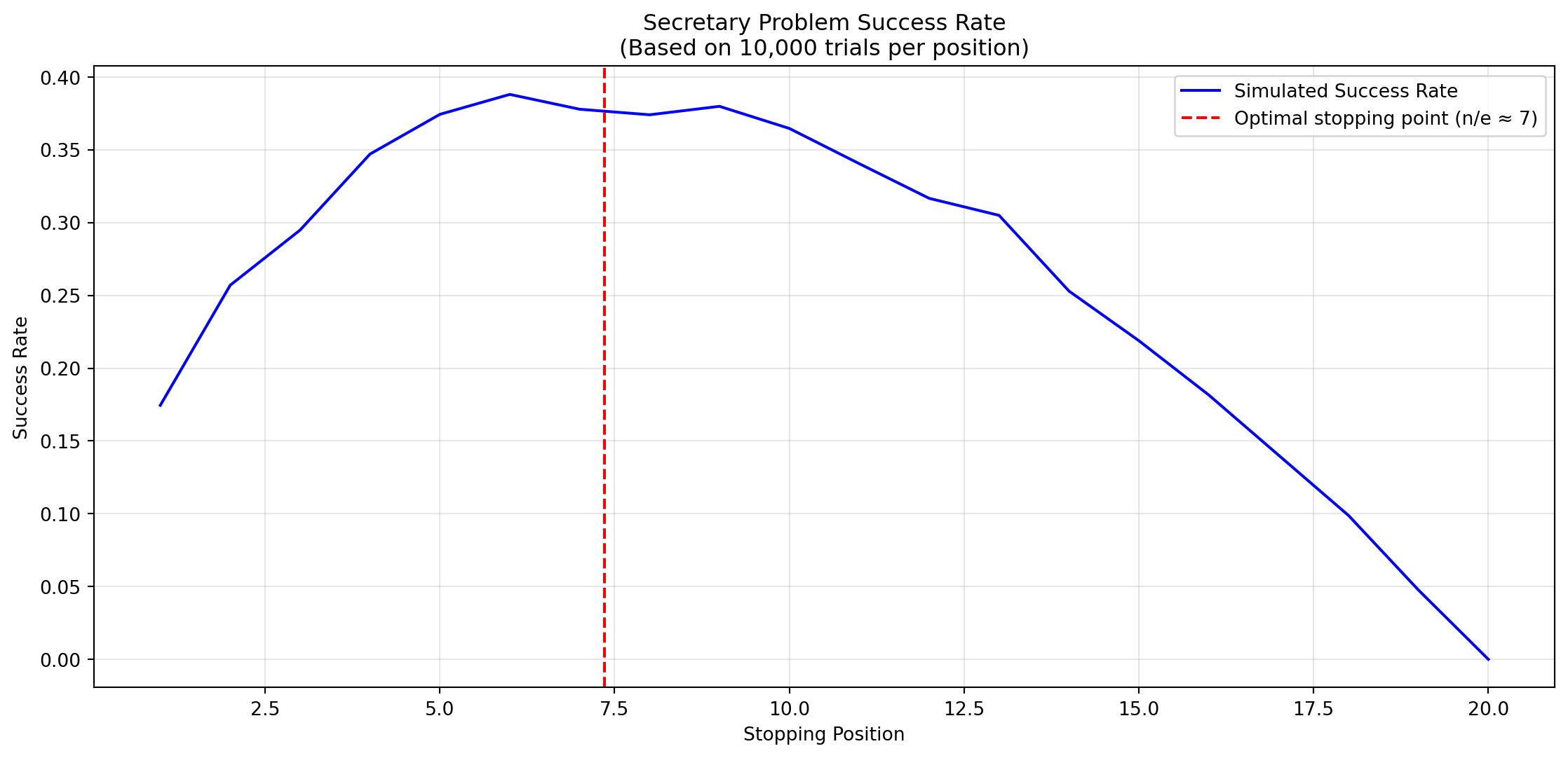
import mathpercentage =1/math.eprint(f"Percentage of options to look at: {percentage:.3f}%")candidates =20lookout_phase = candidates/math.eprint(f"Look at first {lookout_phase:.3f} candidates")
Percentage of options to look at: 0.368%
Look at first 7.358 candidates
. . .
No worries if you don’t understand the code! We are essentialy just using the formula to calculate the percentage of candidates to look at.
Geometric Distribution
Let’s visualize the success of a simulation with 20 candidates:
Variations
Rejection
Question: Imagine a dating scenario, where the other person can also reject you. Optimal stopping point?
The optimal stopping point is now lower
Because we can now fail more often
With 50 % chance of rejection, we start leaping at 25 %
Formula:\(q^{\frac{1}{1-q}}\) with \(q\) being the chance of rejection
Mutual Rejection
Question: What if in dating, the other person can also reject you?
The optimal stopping point decreases
We need to account for rejection risk
With 50% rejection probability: start accepting at 25%
Formula:\(q^{\frac{1}{1-q}}\) where \(q\) = rejection probability
. . .
Life lesson: Higher risk of rejection means we should be less picky!
Time Constraints
What if we don’t have a fixed number of candidates, but a fixed amount of time?
. . .
Example: One year to find an apartment
. . .
Question: How should we adapt our strategy?
. . .
Same principle applies! Observe for first 37% of available time
But now we also control the search intensity
This connects to resource allocation problems in computer science
Other versions
Selling a house for the best price (“Threshold Rule”)
Stealing with a success probability (“Burglar’s Problem”)
Finding a parking spot (“Parking Lot Problem”) [^2]
. . .
Side note for drivers: An increase in occupancy from 90 to 95% doubles the search time for all drivers!
Building Your Technical Mindset
Question:How does optimal stopping connect to programming?
. . .
Algorithmic thinking: Break complex decisions into logical steps
Trade-off analysis: Exploration vs. exploitation (fundamental in AI)
Mathematical optimization: Using formulas to find best solutions
Key Takeaways
What we learned:
Optimal stopping problems are everywhere in life and business
The 37% rule provides a mathematically optimal strategy
Exploration vs. exploitation is a fundamental trade-off
Real-world variations require adapting the basic strategy
This thinking builds foundation for algorithmic problem-solving
Any questions
so far?
After the break — Optimal Stopping
Gentle introduction to Python Programming
We work in our notebooks on basics and optimal stopping
How to translate the idea into code and experiments
. . .
That’s it for optimal stopping!
Let’s have a short break and then continue with our first Python programming session.
Literature
Interesting literature to start
Christian, B., & Griffiths, T. (2016). Algorithms to live by: the computer science of human decisions. First international edition. New York, Henry Holt and Company.3
Ferguson, T.S. (1989) ‘Who solved the secretary problem?’, Statistical Science, 4(3). doi:10.1214/ss/1177012493.
Books on Programming
Downey, A. B. (2024). Think Python: How to think like a computer scientist (Third edition). O’Reilly. Here
Elter, S. (2021). Schrödinger programmiert Python: Das etwas andere Fachbuch (1. Auflage). Rheinwerk Verlag.
. . .
Think Python is a great book to start with. It’s available online for free. Schrödinger Programmiert Python is a great alternative for German students, as it is a very playful introduction to programming with lots of examples.
More Literature
For more interesting literature, take a look at the literature list of this course.
Footnotes
Large number of candidates! With a small number of candidates, we can do even better. . . .↩︎
This is a bit more advanced. We will not go into the details of the math here and focus more on the insights. For more details see Ferguson, T.S. (1989) ‘Who solved the secretary problem?’, Statistical Science, 4(3). doi:10.1214/ss/1177012493.↩︎
The main inspiration for this lecture. Nils and I have read it and discussed it in depth, always wanting to translate it into a course.↩︎