Session 03-04 - Transformations & Graphical Analysis
Section 03: Functions as Business Models
Dr. Nikolai Heinrichs & Dr. Tobias Vlćek
Entry Quiz - 10 Minutes
Review from Session 03-03
Work individually, then we compare together
Find the vertex of \(f(x) = -2x^2 + 12x - 10\) and determine if it’s a maximum or minimum.
A company’s profit function is \(P(x) = -x^2 + 80x - 1200\). Find:
- The quantity that maximizes profit
- The maximum profit
Convert \(g(x) = x^2 - 4x + 7\) to vertex form.
Revenue is modeled by \(R(p) = p(600 - 3p)\). What price maximizes revenue?
Homework Discussion - 20 Minutes
Sharing Solutions from Tasks 03-03
Focus on optimization strategies
- Problem 3: Theater revenue optimization
- How did capacity constraints affect your solution?
- Problem 5: Area optimization with fencing
- Impact of the river (no fence needed)?
- Problem 7: Multi-product optimization (if attempted)
- Bundling vs. separate pricing insights?
Key Insight
Optimization often involves balancing mathematical ideals with practical constraints!
Vertical Transformations
Vertical Shifts
Moving graphs up or down
Given original function \(f(x)\):
- Upward shift: \(g(x) = f(x) + k\) (k > 0)
- Downward shift: \(g(x) = f(x) - k\) (k > 0)
- Graph effect: Entire graph moves vertically
- Business meaning:
- Fixed cost changes
- Base price adjustments
- Overhead modifications
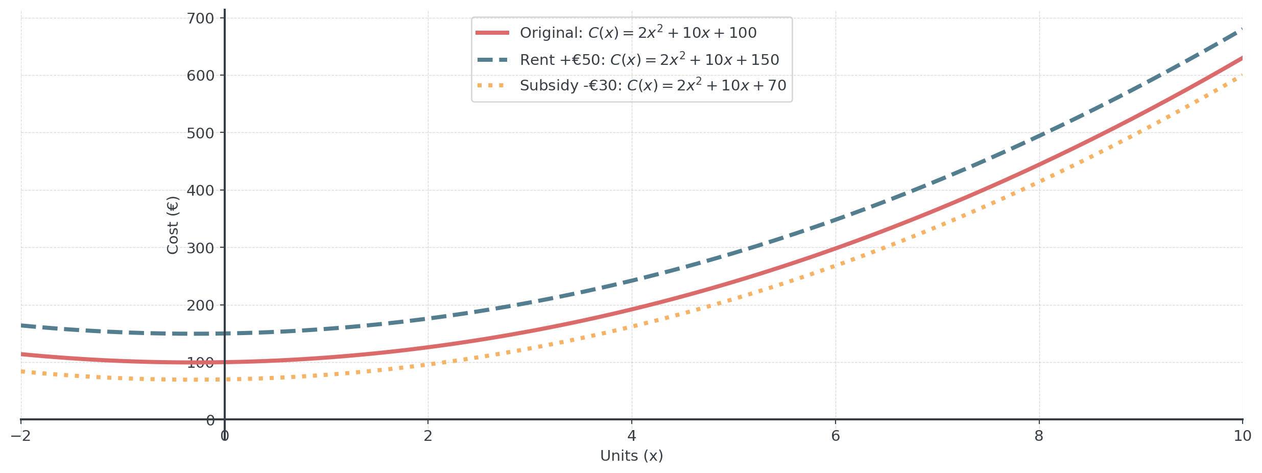
Example: Cost Function Adjustment
Original cost: \(C(x) = 5x^2 + 3x + 100\)
- Rent increases by €100: \(C_{new}(x) = 5x^2 + 3x + 200\)
- Government subsidy of €50: \(C_{new}(x) = 5x^2 + 3x + 50\)
Question: Any idea how we could graph this?
Vertical Shift Visualization
Same parabola shape, shifted vertically - fixed costs change, but variable cost structure remains the same!
Vertical Stretching and Compression
Changing the vertical scale
Given original function \(f(x)\):
- Vertical stretch: \(g(x) = a \cdot f(x)\) where \(a > 1\)
- Vertical compression: \(g(x) = a \cdot f(x)\) where \(0 < a < 1\)
- Reflection: \(g(x) = -f(x)\) (flip over x-axis)
- Business meaning:
- Percentage markups/discounts
- Tax multipliers
- Currency conversions
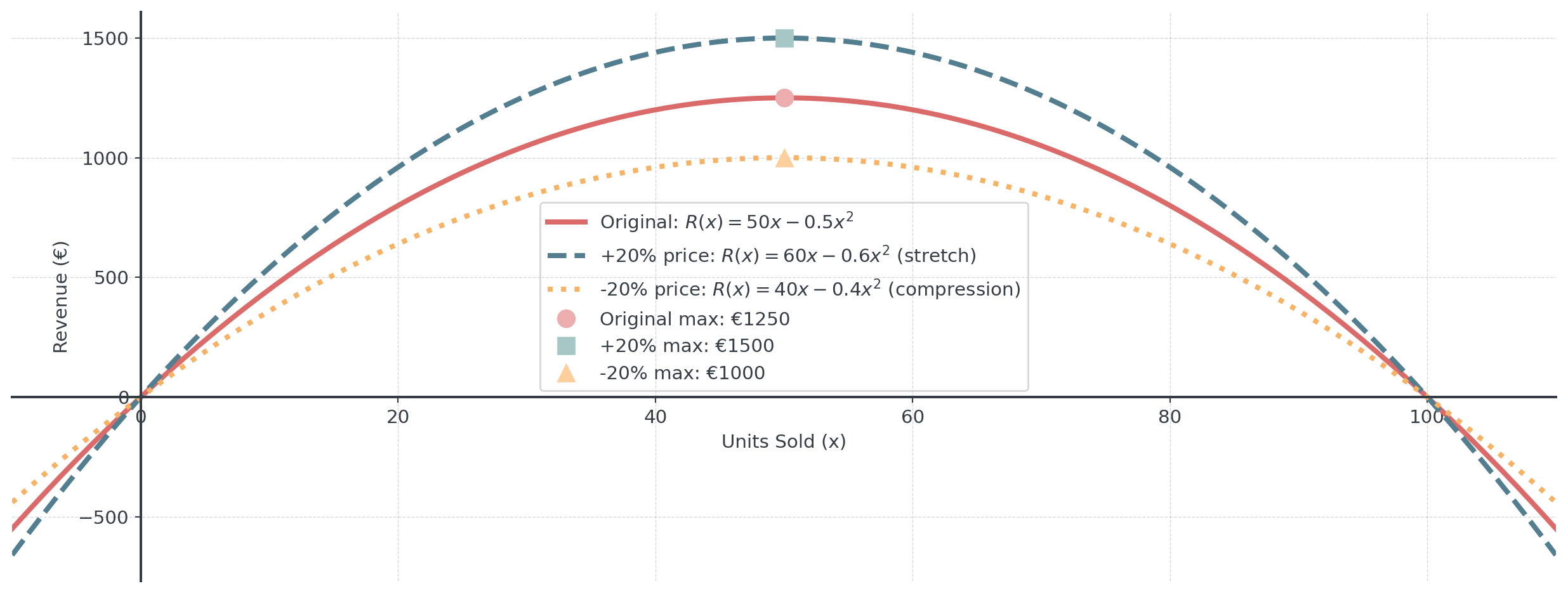
Example: Revenue Scaling
Original revenue: \(R(x) = 50x - 0.5x^2\)
- 20% price increase across all products: \(R_{new}(x) = 1.2(50x - 0.5x^2) = 60x - 0.6x^2\)
- 20% price decrease across all products: \(R_{new}(x) = 0.8(50x - 0.5x^2) = 40x - 0.4x^2\)
Question: Can anyone describe what happens now?
All three functions have the same optimal quantity (50 units), but revenue scales proportionally with price - stretch up or compress down!
Vertical Stretch and Compression
Reflection Visualization
Quick Practice - 10 Minutes
Work individually, then we discuss
Given the original profit function: \(P(x) = -x^2 + 40x - 200\)
- Write the new function if fixed costs increase by €100
- Write the new function if a government grant reduces costs by €50
- Write the new function if all revenues increase by 30%
- Write the new function if all revenues decrease by 25%
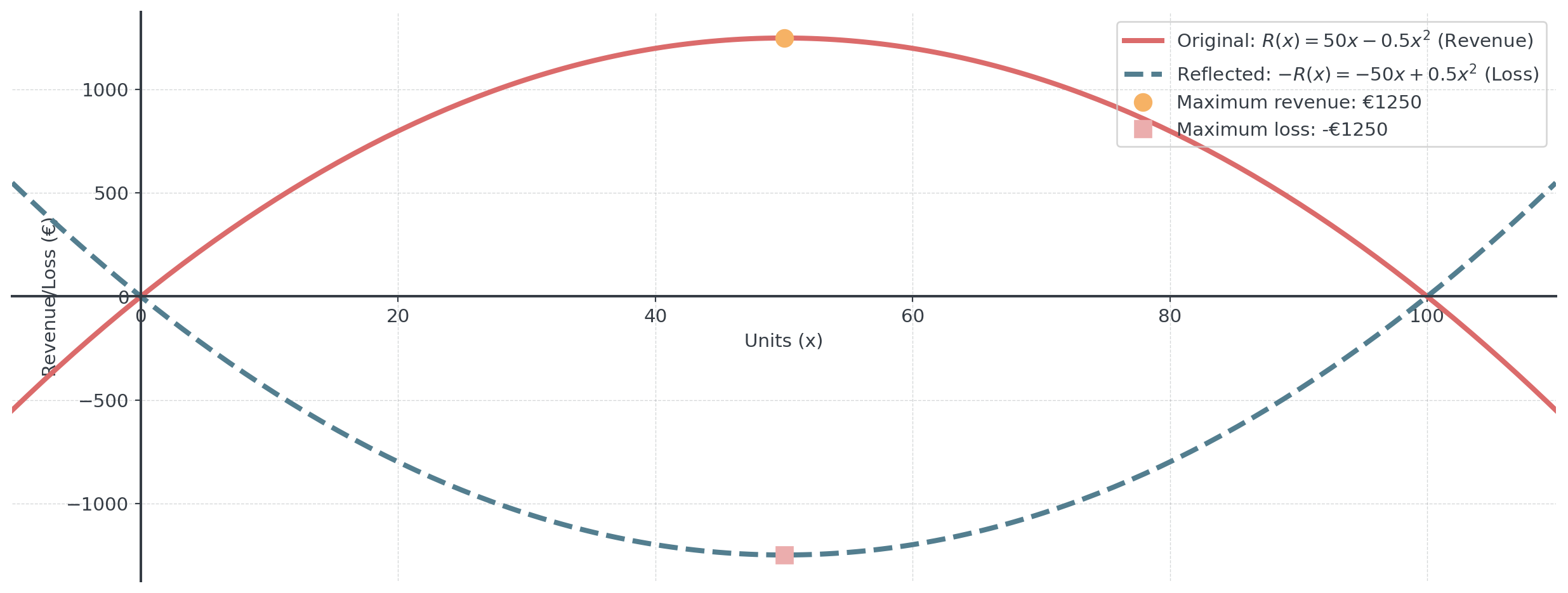
- What business scenario could \(-P(x)\) represent?
- Write the reflected function explicitly
Break - 10 Minutes
Horizontal Transformations
Horizontal Shifts
Moving graphs left or right
Given original function \(f(x)\):
- Right shift: \(g(x) = f(x - h)\) where \(h > 0\)
- Left shift: \(g(x) = f(x + h)\) where \(h > 0\)
- Business meaning:
- Time delays or advances
- Market entry timing
- Seasonal adjustments
Counterintuitive: Minus shifts right, plus shifts left!
Example: Seasonal Demand Shift
Summer demand peaks in June (month 6): \(D(t) = -(t-6)^2 + 100\)
- Unusually hot weather shifts peak to May (left shift): \(D_{new}(t) = -(t-5)^2 + 100\)
- Unusually cold weather shifts peak to July (right shift): \(D_{new}(t) = -(t-7)^2 + 100\)
Question: Anyone with an idea how to graph this?
Same shape parabola, shifted horizontally - peak demand moves but pattern stays the same!
Horizontal Shift Visualization
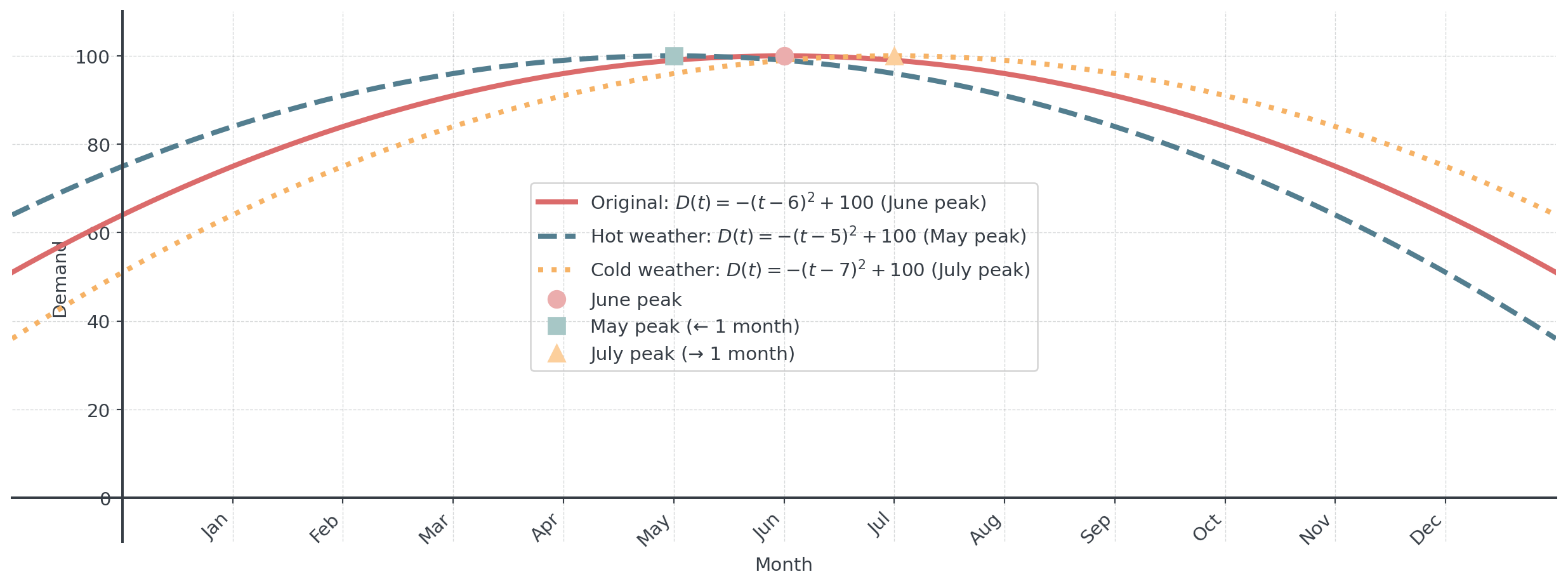
Remember: \(D(t-5)\) shifts RIGHT to May, \(D(t-7)\) shifts RIGHT to July - counterintuitive notation!
Horizontal Stretch and Compression
Changing the horizontal scale
Given original function \(f(x)\):
- Horizontal stretch: \(g(x) = f(x/b)\) where \(b > 1\)
- Horizontal compression: \(g(x) = f(bx)\) where \(b > 1\)
- Reflection: \(g(x) = f(-x)\) (flip over y-axis)
- Business meaning:
- Time scaling (quarterly to monthly)
- Production speed changes
- Market cycle adjustments
Example: Product Lifecycle
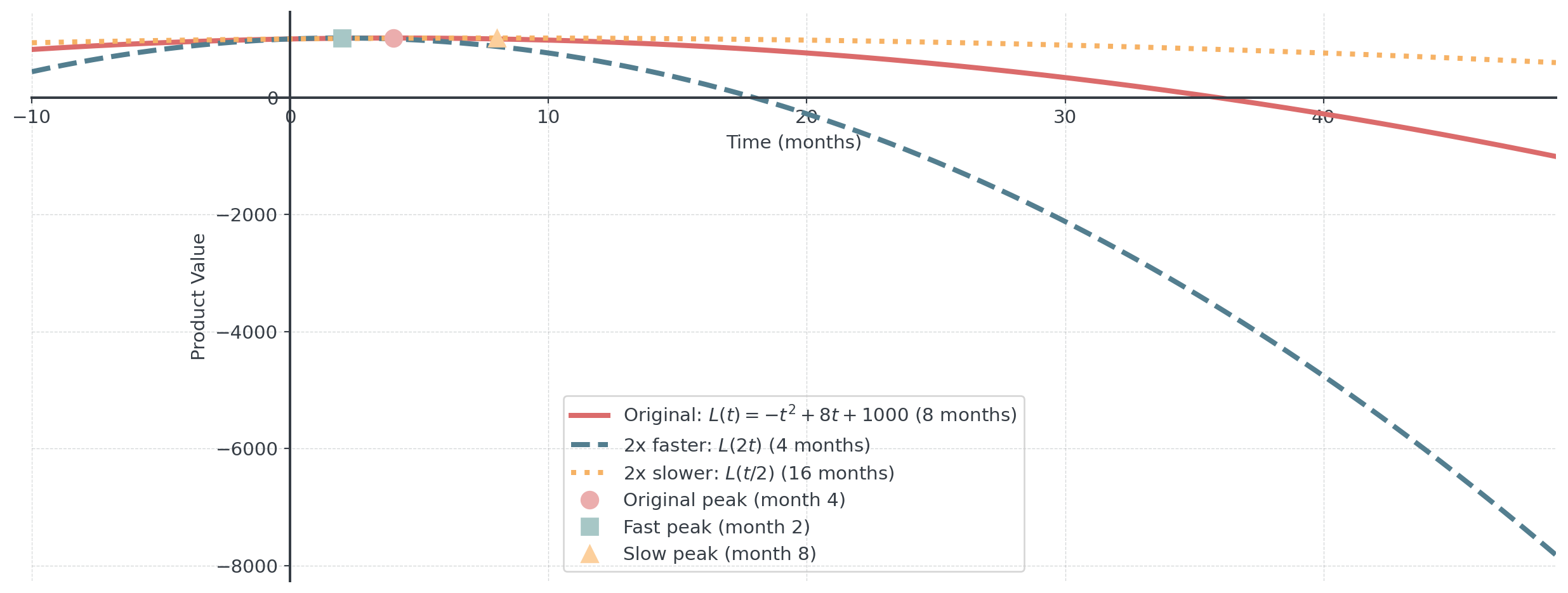
Original lifecycle (monthly): \(L(t) = -t^2 + 8t + 1000\)
- Competitor speeds up cycle (2x faster): \(L_{fast}(t) = -(2t)^2 + 8(2t) = -4t^2 + 16t + 1000\)
- Extended warranty slows cycle (2x slower): \(L_{slow}(t) = -(t/2)^2 + 8(t/2) = -0.25t^2 + 4t + 1000\)
Question: What happens to the lifecycle duration?
Horizontal compression (faster) → narrower curve, earlier peak.
Horizontal stretch (slower) → wider curve, later peak!
Counterintuitive again: \(f(2t)\) compresses (faster), \(f(t/2)\) stretches (slower)!
Horizontal Stretch/Compression
Combining Transformations
Order of Operations
Apply transformations systematically
Standard order for \(g(x) = a \cdot f(b(x - h)) + k\):
- Horizontal shift by \(h\)
- Horizontal stretch/compress by factor \(b\)
- Vertical stretch/compress by factor \(a\)
- Vertical shift by \(k\)
Let’s apply these steps to a function!
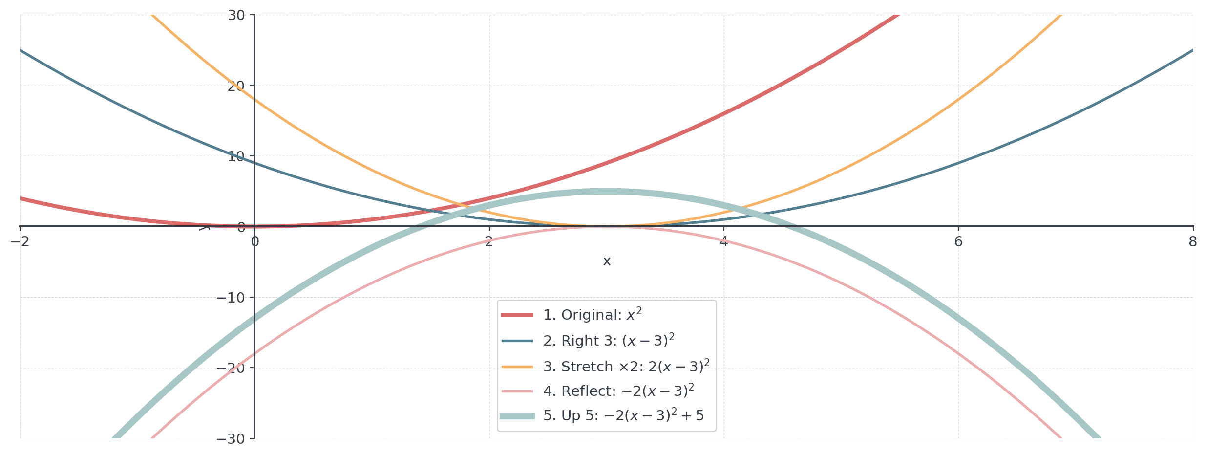
Complete Transformation Example
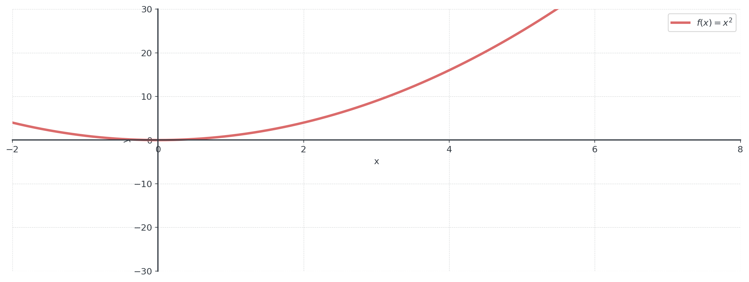
Start with \(f(x) = x^2\)
Transform to: \(g(x) = -2(x - 3)^2 + 5\)
- Shift right 3 units: \((x - 3)^2\)
- Stretch vertically by 2: \(2(x - 3)^2\)
- Reflect over x-axis: \(-2(x - 3)^2\)
- Shift up 5 units: \(-2(x - 3)^2 + 5\)
Question: Who can describe how this might look like?
Original Function
Progressive Transformation
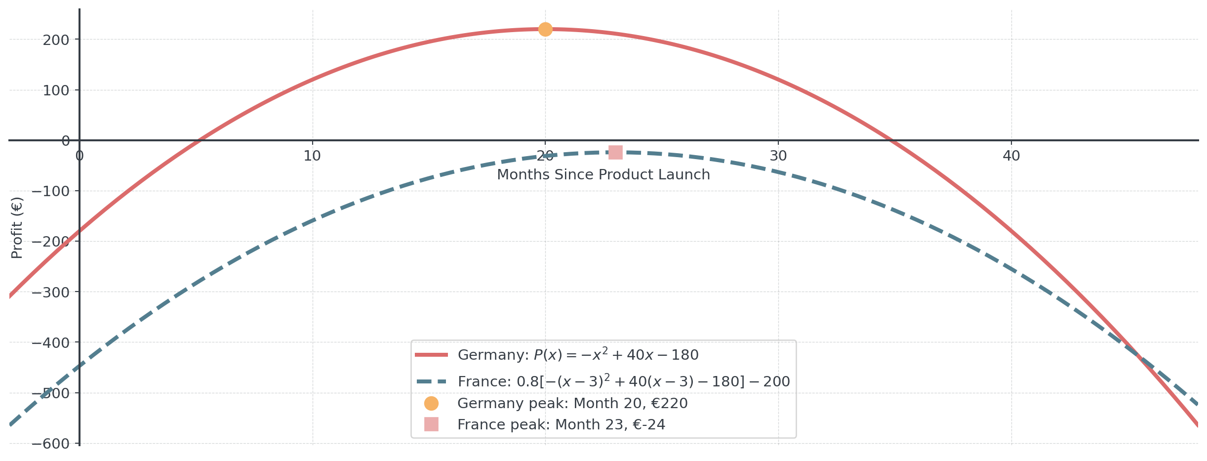
Business Scenario: Market Expansion
Original profit in Germany: \(P(x) = -x^2 + 40x - 180\)
Research estimates expansion to France with adjustments:
- 20% higher costs: Multiply by 0.8
- Fixed cost increase of €200: Subtract 200
- 3-month delay: Replace \(x\) with \((x - 3)\)
- \(P_{France}(x) = 0.8[-(x-3)^2 + 40(x-3) - 180] - 200\)
Question: Should the company expand to France?
Market Expansion Visualization
Guided Practice
Individual Exercise Block I
Work alone for 10 minutes, then we discuss the solutions
Given \(f(x) = x^2 - 4x + 3\), write the equation for:
- \(f(x)\) shifted up 5 units
- \(f(x)\) shifted left 2 units
- \(f(x)\) reflected over the x-axis
A cost function is \(C(x) = 0.5x^2 + 20x + 500\). Due to inflation:
- All costs increase by 10%
- An additional fixed cost of €100 is added
- Write new cost function and find cost for producing 50 units.
Individual Exercise Block II
Work alone for 5 minutes, then we discuss the solutions
- The demand for ice cream follows \(D(t) = -2(t - 7)^2 + 200\) where \(t\) is the month.
- In which month is demand highest?
- If climate change shifts the peak 1 month earlier and increases maximum demand by 15%, write the new function.
Coffee Break - 15 Minutes
Reading Economic Graphs
Extracting Information from Graphs
Graphs tell business stories
Key features to identify:
- Intercepts: Starting values, break-even points
- Slope/Rate of change: Marginal values, trends
- Maximum/Minimum: Optimal points, extremes
- Intersections: Equilibrium, equal values
- Shape: Linear, quadratic, exponential growth patterns
- Domain/Range: Feasible regions, constraints
Graph Analysis Example
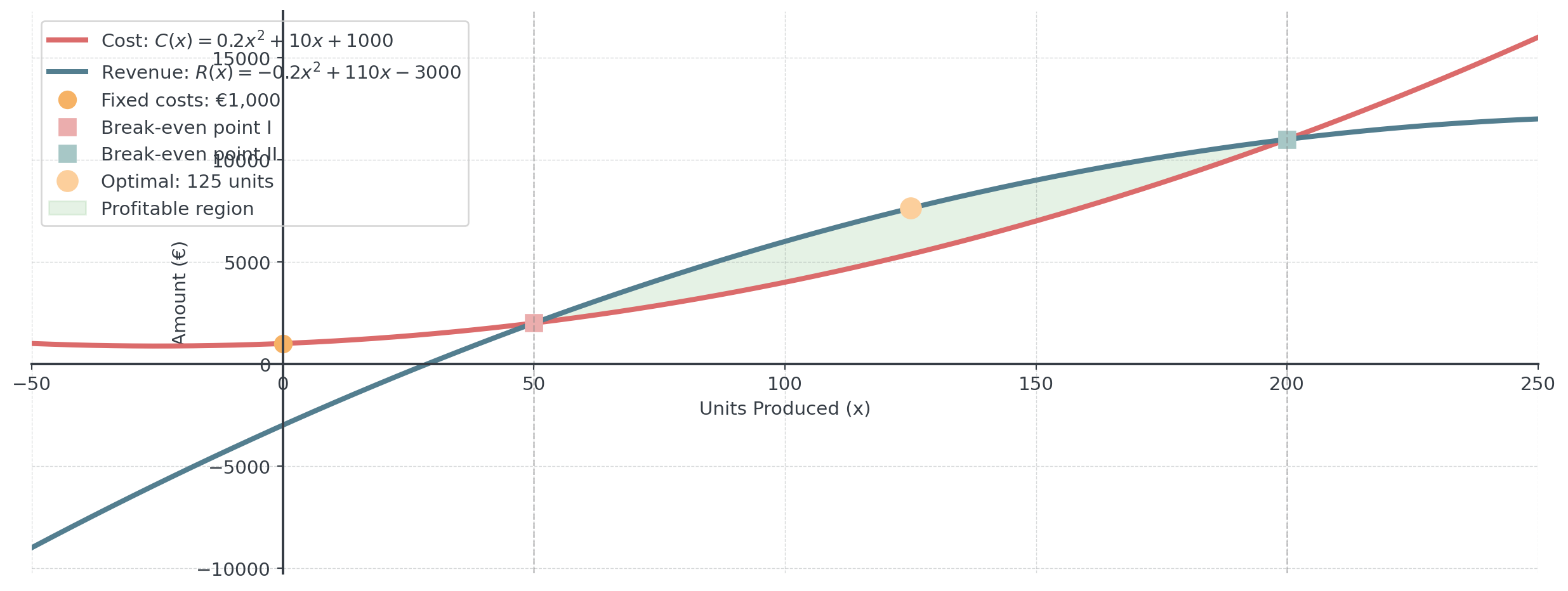
Scenario: A graph shows two curves:
- Cost function: Starts at (0, 1000), curves upward
- Revenue function: Starts at origin, curves then flattens
- They intersect at x = 50 and x = 200
Business insights:
- Fixed costs: €1,000 (y-intercept of cost)
- Break-even points: 50 and 200 units
- Profitable region: Between 50 and 200 units
- Optimal production: Where vertical distance is maximum
Visualizing the Business Story
Comparative Graph Analysis
Comparing multiple scenarios visually
When comparing functions:
- Parallel lines: Same variable costs, different fixed costs
- Different slopes: Different efficiency levels
- Intersection points: Crossover quantities
- Vertical distances: Profit or loss amounts
Collaborative Problem-Solving
Franchise Expansion Analysis
The Scenario: Coffee Chain Expansion
A successful coffee shop has this profit model for their original location: \[P(x) = -0.1x^2 + 50x - 4000\] where \(x\) is the number of customers per day.
Understanding the function:
- The \(-0.1x^2\) term represents diminishing returns (congestion, slower service)
- The \(50x\) term represents revenue per customer
- The \(-4000\) represents daily fixed costs
Now, they want to open franchises in different markets!
Transformation Hints
- Revenue changes affect the \(50x\) coefficient
- Fixed cost changes affect the \(-4000\) constant
- Efficiency changes affect the \(-0.1x^2\) coefficient (less negative = more efficient)
- Vertical scaling multiplies the entire function
The Different Markets
- Revenue: 30% higher prices → multiply \(50x\) by 1.3
- Fixed costs: Increase by €1,000 → change \(-4000\) to \(-5000\)
- Efficiency: Same as original
Task: Apply these transformations to get \(P_A(x)\)
- Revenue: Same per customer (\(50x\) unchanged)
- Efficiency: Better workflow reduces congestion → multiply \(-0.1x^2\) by 0.8 (less negative)
- Fixed costs: Increase by €2,000 → change \(-4000\) to \(-6000\)
Task: Apply these transformations to get \(P_B(x)\)
- Revenue: 40% lower prices → multiply \(50x\) by 0.6
- Fixed costs: Decrease by €500 → change \(-4000\) to \(-3500\)
- Efficiency: Same as original
Task: Apply these transformations to get \(P_C(x)\)
Your Tasks
Work in groups of 3-4 students
Write the transformed profit function for each location
Find the optimal number of customers for each location
Calculate the maximum daily profit for each location
Which location should be prioritized for expansion and why?
If the company can afford total fixed costs of €15,000 per day across all locations (including original), which combination of locations should they operate?
Wrap-Up
Key Takeaways
- Vertical shifts represent fixed changes
- Horizontal shifts represent timing changes
- Stretches and compressions show scaling effects
- Multiple transformations model complex scenarios
- Graphs reveal optimization opportunities
- Business decisions require comprehensive analysis
Final Assessment
5 minutes - Individual work
A retailer’s monthly profit is modeled by \(P(x) = -2x^2 + 100x - 800\) where \(x\) is the number of items sold in hundreds.
Due to economic changes:
- A competitor enters, reducing maximum profit by 25%
- Break-even point shifts from 10 to 15 items (hundreds)
- What transformation represents the competitor’s impact?
- What transformation represents the break-even shift?
- Sketch how the graph would change.
Next Session Preview
Session 03-05: Composition, Inverses & Advanced Graphing
- Function composition for multi-step processes
- Finding inverse functions
- When are functions invertible?
- Advanced graphing techniques
- Complex business process modeling
Homework Assignment: Complete Tasks 03-04!
Appendix
Comparing All Locations
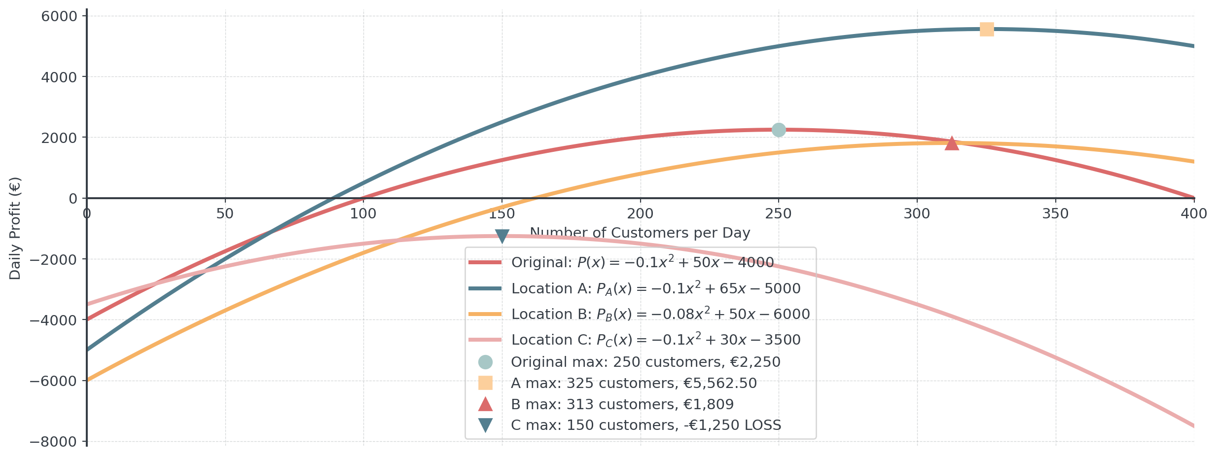
Location A is the clear winner! Location C never breaks even - avoid it despite lower fixed costs!
Session 03-04 - Transformations & Graphical Analysis | Dr. Nikolai Heinrichs & Dr. Tobias Vlćek | Home