Forecasting the Future

Lecture 5 - Management Science

Dr. Tobias Vlćek

Introduction

Client Briefing: MegaMart Retail Chain

Operations Director’s Crisis:

“Last Christmas, we ran out of PlayStation 5s but had 500 unsold fitness trackers. We lost €2M in missed sales and clearance losses. How do we predict what customers will actually buy?”

Business: The Unknown Future

Question: Why can’t we just order the same as last year?

Market: New products, competition
Seasonal Shifts: Weather, holidays, economic conditions
Trend Changes: Changing preferences, new technologies
Randomness: Viral TikToks, supply chain disruptions, pandemics

Reality: Large retailers process several thousand orders per hour. Each stockout basically means lost revenue + unhappy customers.

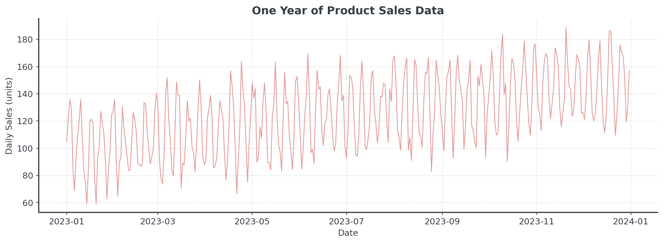
Hidden Patterns in Data

Look at this daily sales data. What patterns do you see?

Core Concepts

Decomposing Time Series

Time series can often be decomposed:

\[Y_t = T_t + S_t + R_t\]

Where:

\(Y_t\) = Observed value at time t
\(T_t\) = Trend component
\(S_t\) = Seasonal component
\(R_t\) = Random/Residual component

Additive vs Multiplicative Models

How do the components combine?

Additive Model \[Y_t = T_t + S_t + R_t\]

Seasonal fluctuations are constant
“We always sell 200 extra in December”
Good: Stable, mature products

Multiplicative Model \[Y_t = T_t \times S_t \times R_t\]

Seasonal fluctuations scale with trend
“December sales are 40% higher”
Good: Growing businesses

Visual Decomposition

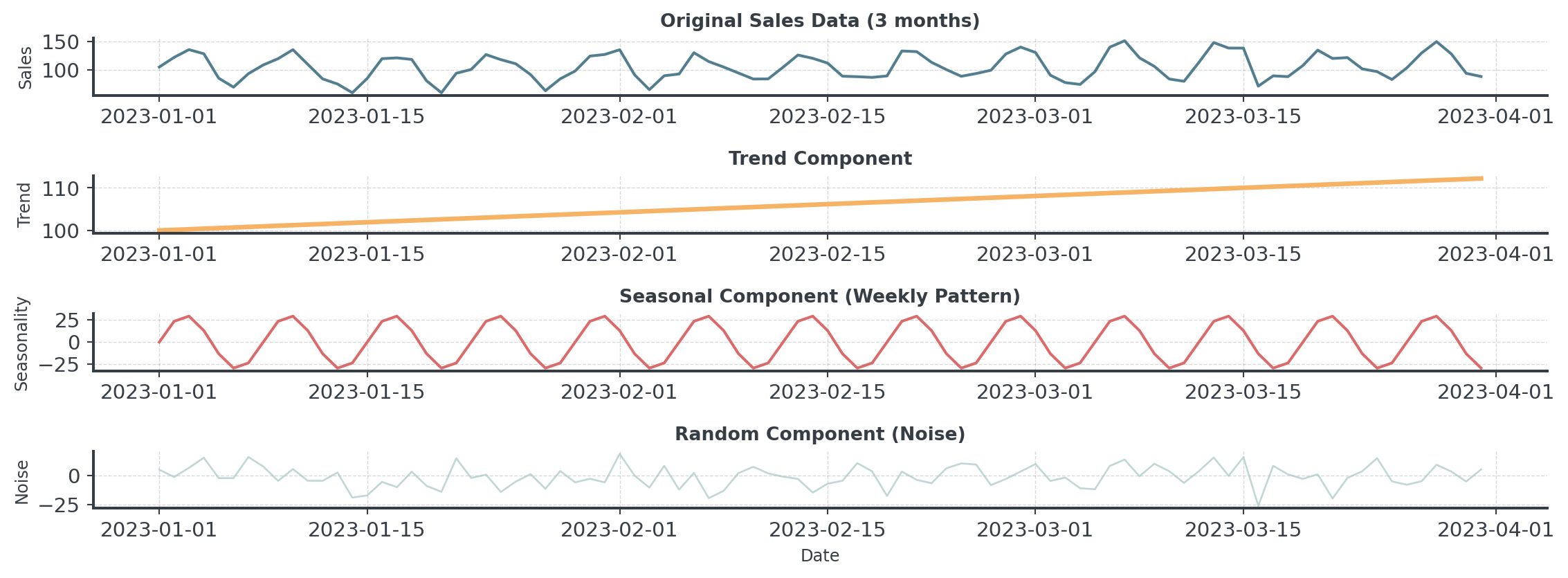
Here: Sales = Trend + Seasonality + Random Noise

Moving Average

Question: How do we separate signal from noise?

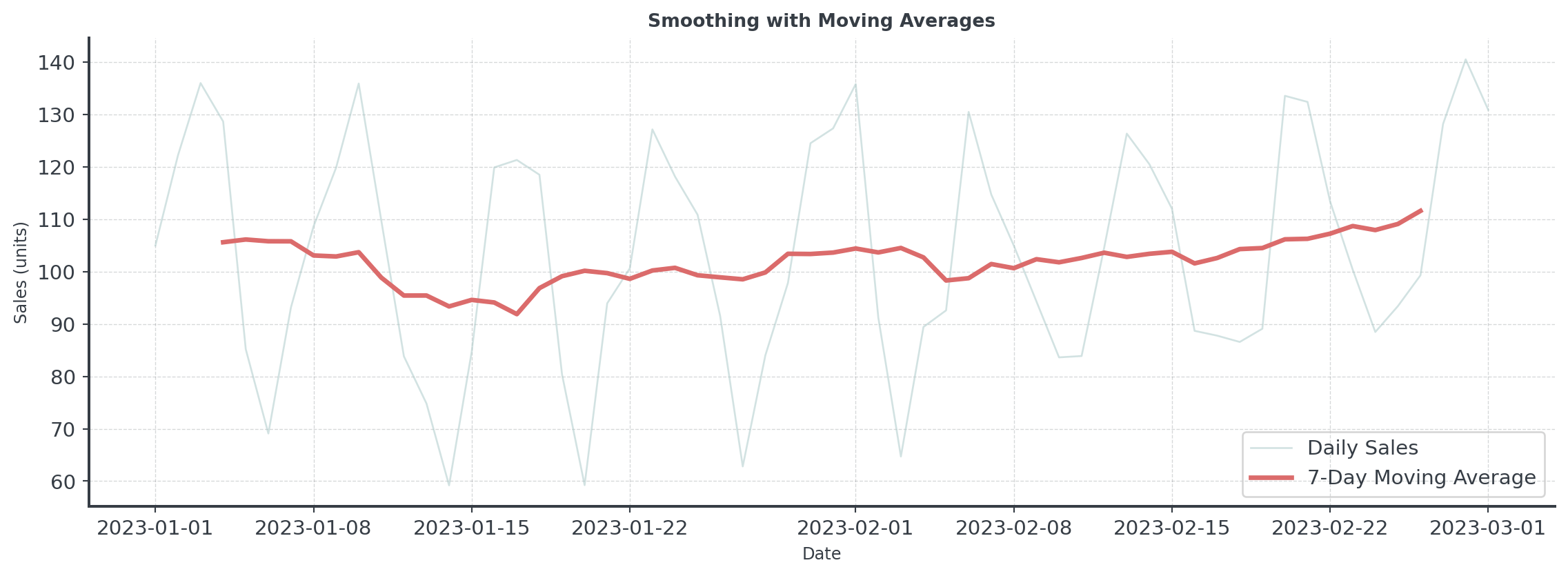
Simple vs Weighted Averages

Which forecast would you trust more?

Simple Moving Average

All days equally important
We just take the average
[14, 15, 16, 14, 15, 16, 17]
Forecast: 15.3

Weighted Moving Average

Recent days matter more
Days closer are weighted more
[0.05, 0.05, 0.1, 0.1, 0.2, 0.2, 0.3]
Forecast: 15.9

Recent data often predicts the future better than old data!

Exponential Smoothing Methods

Simple Exponential Smoothing

Not too simple, not too complex

\[\text{Forecast}_{t+1} = \alpha \times \text{Actual}_t + (1-\alpha) \times \text{Forecast}_t\]

α (alpha) = smoothing parameter (0 to 1)
α = 0.9: Trust recent data (reactive)
α = 0.1: Trust historical patterns (stable)
α = 0.3: Balanced approach (common default)

Think of \(\alpha\) like: How much do you trust the latest data point?

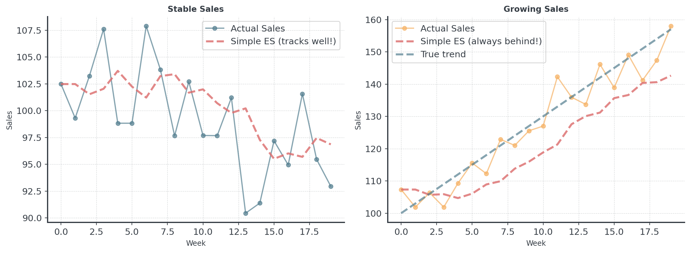
When Simple Smoothing Fails

Simple smoothing assumes the data is flat. What if it’s not?

Adding Trend

Holt’s Method: The Idea

Track TWO things separately: Level and Trend

Level (L): Where are we right now? (like simple ES)
Trend (b): How fast are we growing/declining per period?
Forecast: Combine both: Level + (Trend × periods ahead)

Why This Works:

Simple ES only tracks level (current position)
Holt’s also tracks the slope (direction and speed)

Think of driving a car: Simple ES only knows your position. Holt’s also knows your speed!

Holt’s Method: The Math I

The formulas (simplified for intuition):

Level Equation: \[L_t = \alpha \times Y_t + (1-\alpha) \times (L_{t-1} + b_{t-1})\]

Trend Equation: \[b_t = \beta \times (L_t - L_{t-1}) + (1-\beta) \times b_{t-1}\]

Forecast Equation: \[\hat{Y}_{t+h} = L_t + h \times b_t\]

Holt’s Method: The Math II

In plain English

Level: “Smooth current observation with previous forecast”
Trend: “Smooth the change in level with our previous trend”
Forecast: “Start at current, add trend for each period ahead”

Not too complicated, right?

Step-by-Step I

Let’s walk through 6 periods manually to build intuition

# Sample data with clear upward trend
sales_data = np.array([100, 105, 112, 118, 124, 130])

# Parameters
alpha = 0.3  # Level smoothing
beta = 0.2   # Trend smoothing

# Initialize
level = sales_data[0]  # Start at first observation
trend = sales_data[1] - sales_data[0]  # Initial trend estimate

print(f"Period 1: Level={level:.1f}, Trend={trend:.1f}")

# Store level and trend history for visualization
level_history = [level]
trend_history = [trend]

Period 1: Level=100.0, Trend=5.0

Step-by-Step II

# Apply Holt's method for periods 2-6
for t in range(1, len(sales_data)):
    # Update level
    prev_level = level
    level = alpha * sales_data[t] + (1 - alpha) * (prev_level + trend)

    # Update trend
    trend = beta * (level - prev_level) + (1 - beta) * trend

    # Store for visualization
    level_history.append(level)
    trend_history.append(trend)

    print(f"Period {t+1}: Sales={sales_data[t]}, Level={level:.1f}, Trend={trend:.1f}")

Period 2: Sales=105, Level=105.0, Trend=5.0
Period 3: Sales=112, Level=110.6, Trend=5.1
Period 4: Sales=118, Level=116.4, Trend=5.3
Period 5: Sales=124, Level=122.4, Trend=5.4
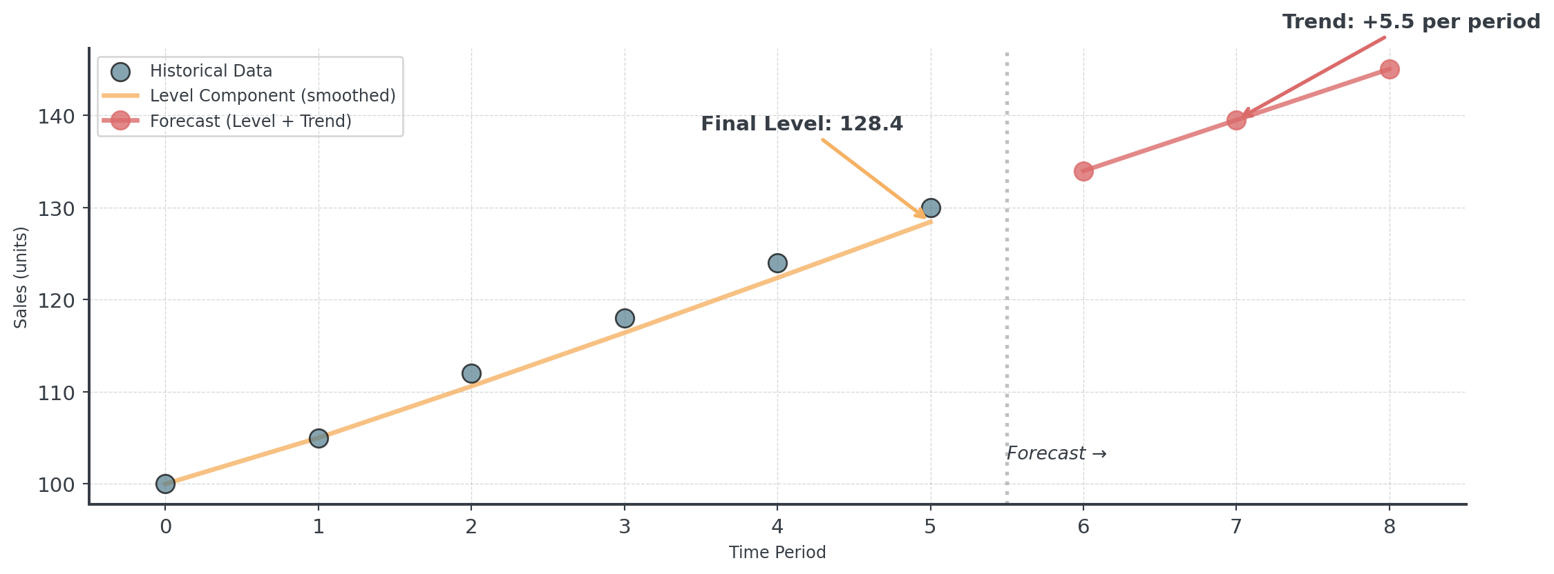
Period 6: Sales=130, Level=128.4, Trend=5.5

Step-by-Step III

# Forecast next 3 periods
print(f"\nForecasts:")
forecast_values = []
for h in range(1, 4):
    forecast = level + h * trend
    forecast_values.append(forecast)
    print(f"  Period {len(sales_data)+h}: {forecast:.1f} units")


Forecasts:
  Period 7: 134.0 units
  Period 8: 139.5 units
  Period 9: 145.0 units

Holt’s Method: Visual Comparison

Choosing Alpha and Beta

How do you pick the right smoothing parameters?

Alpha (Level Smoothing)

High α (0.7-0.9): Responsive
- Use: Volatile markets
Low α (0.1-0.3): Stable
- Use: Steady business

Beta (Trend Smoothing)

High β (0.5-0.8): Quickly
- Use: Dynamic growth/decline
Low β (0.1-0.3): Stable trend
- Use: Consistent growth

Best Practice: Let the algorithm optimize parameters automatically!

You can implement Holt’s method using Python’s statsmodels library!

When to Use

Question: When should you use Holt’s method?

Clear upward or downward trend
No seasonal patterns

Question: When should you use NOT Holt’s method?

Data is flat (use simple ES instead)
Strong seasonality present
Trend direction changes frequently

Adding Seasonality

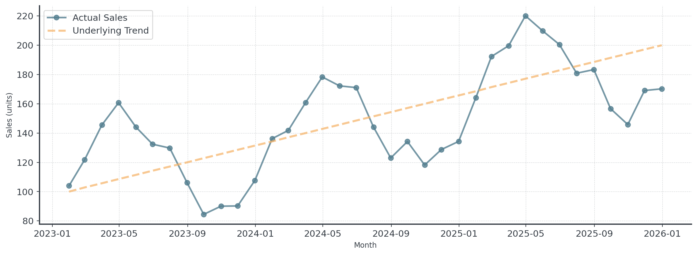
The Problem: Trend + Seasonality

What if your data has BOTH trend AND seasonality?

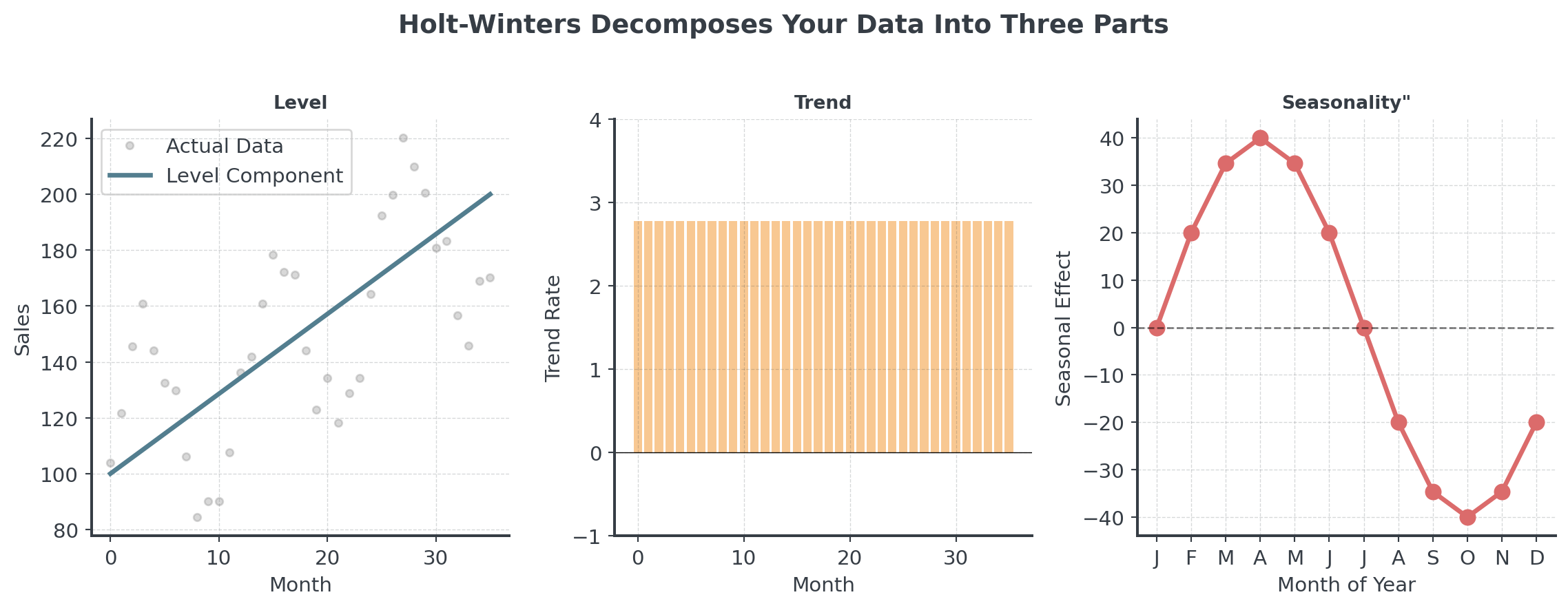
Holt-Winters: Three Components

Track THREE things separately: Level, Trend, AND Seasonality

Level (L): Current baseline demand (deseasonalized)
Trend (b): Growth rate per period
Seasonal Indices (s): Multipliers for each season

Holt-Winters Visualized

Seasonality

How does seasonality combine with the level?

Additive Model \[Y_t = L_t + b_t + s_t\]

Seasonal variation is constant
“We sell +50 units every December”
Pattern: ±constant amount

Multiplicative Model \[Y_t = L_t \times b_t \times s_t\]

Seasonal variation scales with level
“December is 1.5× normal sales”
Pattern: ×percentage change

Holt-Winters: The Math I

The formulas (don’t panic - Python does this for you!)

Additive Model:

\[L_t = \alpha(Y_t - s_{t-m}) + (1-\alpha)(L_{t-1} + b_{t-1})\] \[b_t = \beta(L_t - L_{t-1}) + (1-\beta)b_{t-1}\] \[s_t = \gamma(Y_t - L_t) + (1-\gamma)s_{t-m}\] \[\hat{Y}_{t+h} = L_t + hb_t + s_{t+h-m}\]

Holt-Winters: The Math II

In plain English

Level: Remove seasonality from observation, then smooth
Trend: Same as Holt’s method
Seasonal: Update the seasonal index for this period
Forecast: Level + trend + seasonal adjustment

Parameters:

\(\alpha\) (level), \(\beta\) (trend), \(\gamma\) (seasonal), m (seasonal period length)

Holt-Winters: Intuition I

Understanding seasonal patterns with quarterly sales

Quarterly Sales Pattern:

Q1: Low season (after holidays) → Factor: 0.85
Q2: Spring pickup → Factor: 0.95
Q3: Summer growth → Factor: 1.05
Q4: Holiday peak! → Factor: 1.15

Holt-Winters: Intuition I

How Holt-Winters Works

Deseasonalize the data (remove seasonal effect)
Calculate trend from deseasonalized data
Update seasonal indices based on actual vs. expected
Forecast by combining level + trend + seasonal pattern

Q4 is typically 35% higher than Q1 in retail! Holt-Winters captures this automatically.

Holt-Winters: Visual

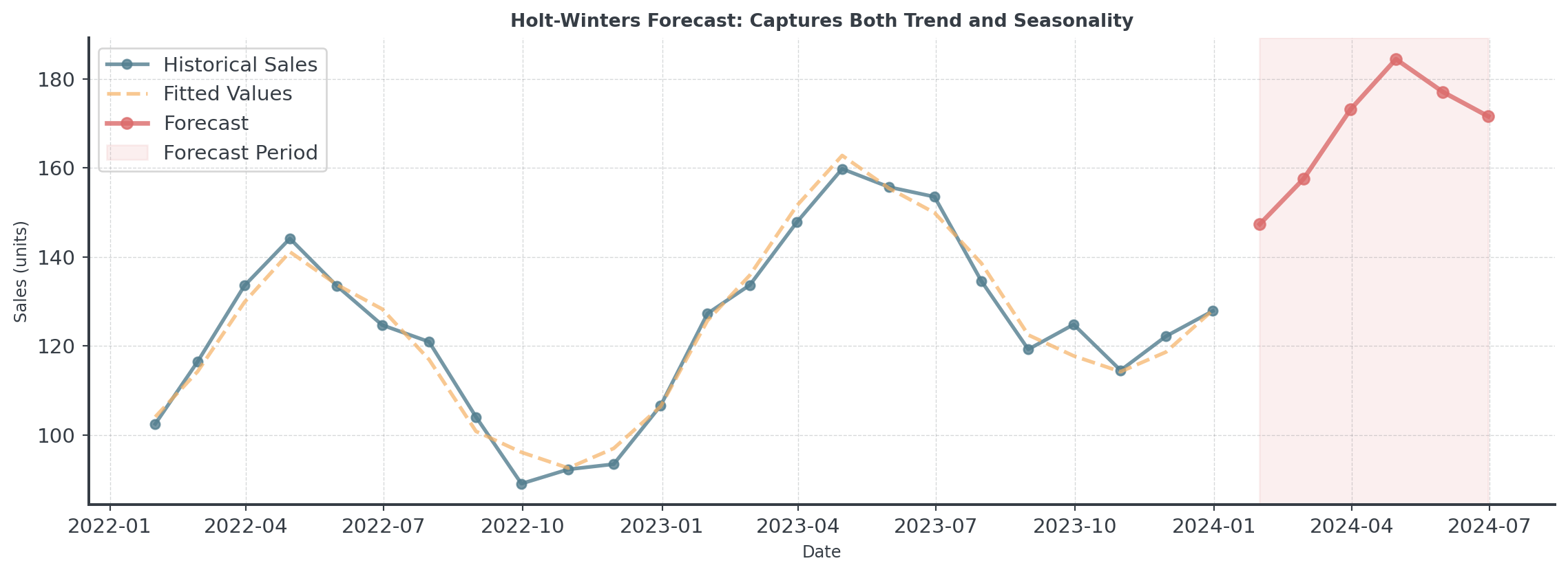
Notice how the forecast continues the seasonal pattern while following the trend!

When to Use Holt-Winters

Question: When should you use Holt-Winters method?

Data with trend AND seasonality
At least 1 full seasonal cycle (2 are better!)
Regular, repeating patterns

Question: When should you AVOID Holt-Winters method?

Irregular or changing seasonal patterns
Flat data with no trend
Seasonal pattern length unknown

Method Selection & Validation

Measuring Forecast Accuracy

How wrong were we?

Mean Absolute Error (MAE): Average size of mistakes \[\text{MAE} = \frac{1}{n} \sum_{i=1}^{n} |Actual_i - Forecast_i|\]

Root Mean Squared Error (RMSE): Penalizes large errors more \[\text{RMSE} = \sqrt{\frac{1}{n} \sum_{i=1}^{n} (Actual_i - Forecast_i)^2}\]

Forecast Accuracy

Easy with Python

# Example: Compare two forecasting methods
actual = np.array([100, 105, 110, 108, 112])
forecast_a = np.array([98, 107, 109, 110, 111])
forecast_b = np.array([102, 103, 112, 106, 113])

mae_a = np.mean(np.abs(actual - forecast_a))
mae_b = np.mean(np.abs(actual - forecast_b))

print(f"Method A - MAE: {mae_a:.2f} units")
print(f"Method B - MAE: {mae_b:.2f} units")
print(f"\nBetter method: {'A' if mae_a < mae_b else 'B'}")

Method A - MAE: 1.60 units
Method B - MAE: 1.80 units

Better method: A

When to Use Which Method?

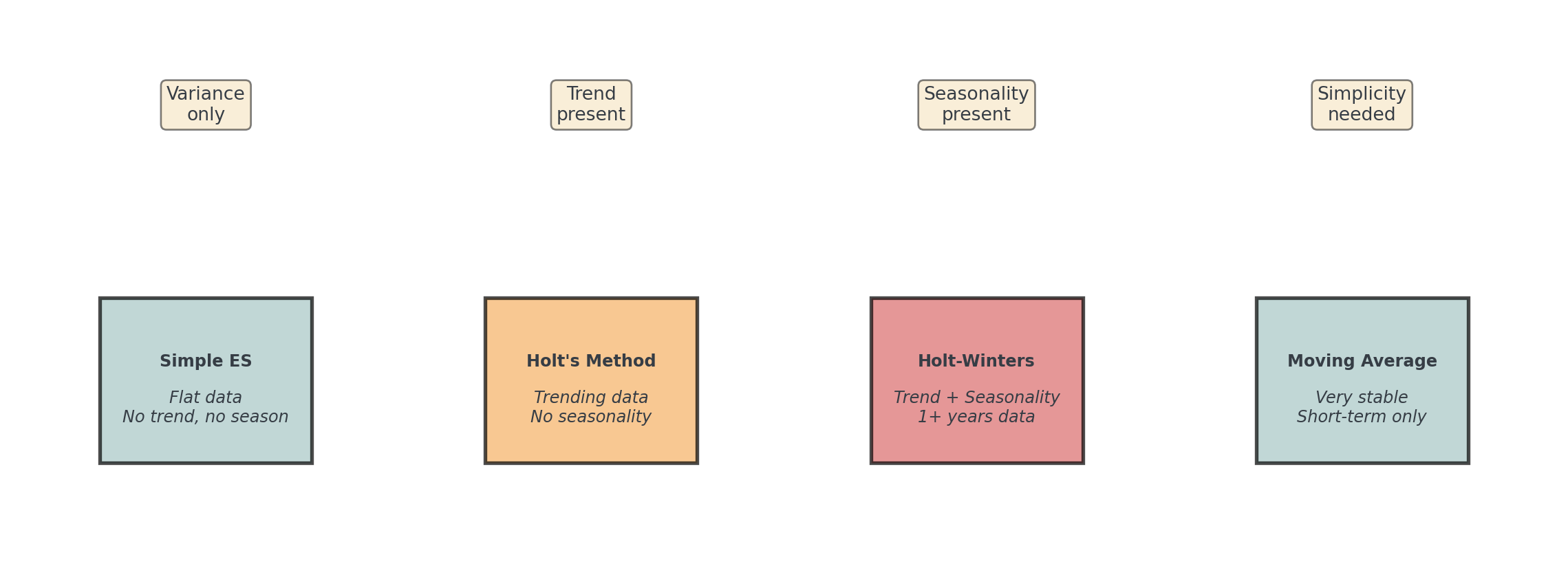
Start simple: Try moving average first as baseline, then add complexity only if needed!

The Real Cost of Being Wrong

Not all forecast errors are equal!

Example: Winter Coats

Cost: €50, Selling Price: €150, Margin: €100
Storage cost: €5/month
Clearance markdown: 70% off

Question: What is your intuition here?

Under and Overforecasting

Sometimes it’s cheaper to overstock than to miss sales!

Underforecast by 100 units:

Lost profit: 100 × €100
- €10,000
Customer disappointment
Competitor gains market share

Overforecast by 100 units:

Storage: 100 × €5 × 3 months
- €1,500
Clearance loss: 100 × €70
- €7,000

The “best” forecast depends on your business context.

Method Implementation

Your Python Practice Notebook

All the hands-on coding happens in the interactive tutorial!

Working with dates in Pandas
Implementing moving averages
Building forecast functions
Applying Holt’s method
Using Holt-Winters
Measuring accuracy

The notebook guides you step-by-step through Bean Counter’s seasonal demand forecasting challenge!

AI & Machine Learning Forecasting

The Promise of AI

Can machines predict better than classical methods?

What AI/ML brings to forecasting:

Handle hundreds of variables simultaneously
Detect complex non-linear patterns
Learn from massive datasets
Adapt automatically to changes

AI doesn’t replace human judgment, it augments it when you have enough data!

Common AI/ML Forecasting

Overview of popular techniques

Traditional ML:

Random Forest: Ensemble of decision trees
XGBoost: Gradient boosting (very popular)
Support Vector Machines: Pattern recognition

Deep Learning:

LSTM (Long Short-Term Memory): For sequences
Prophet (Facebook): Automated forecasting
Neural Networks: Complex patterns

More complex ≠ Better! Simple methods often win in forecasting.

The Issue: Overfitting

Question: What happens when we train an AI on all our data and use it to predict… the same data?

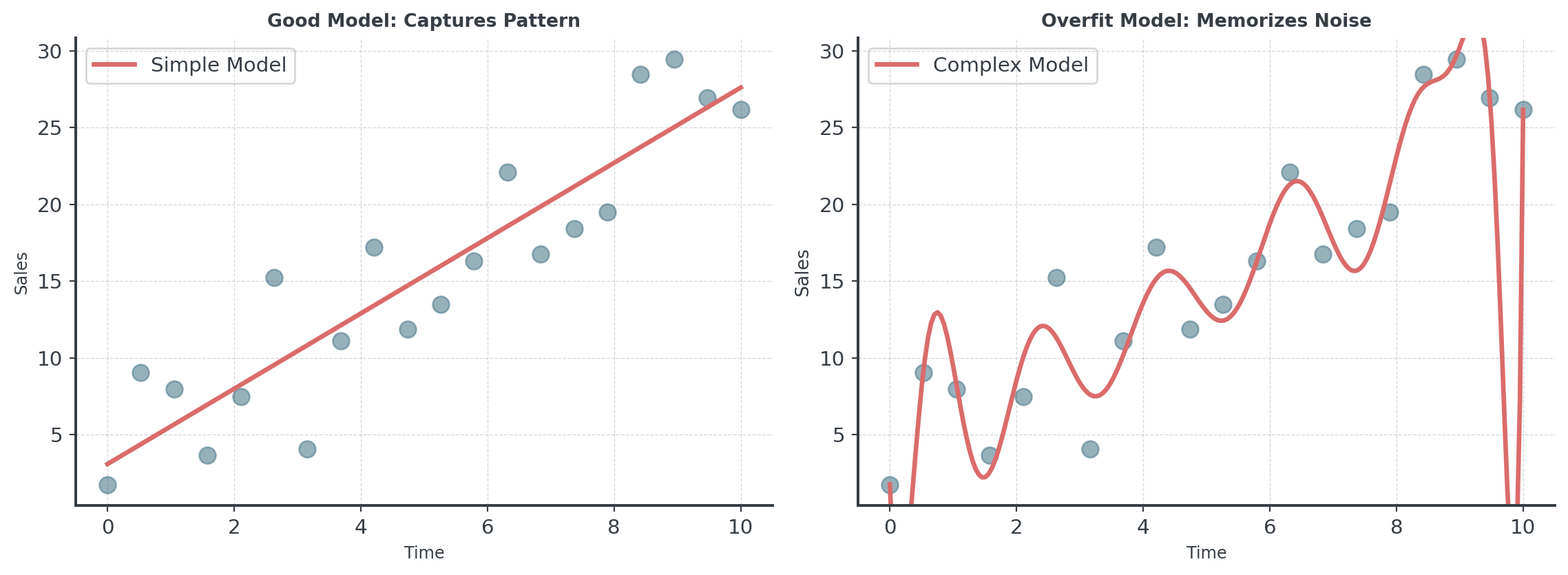
Training vs Test Data

Never judge a complex model on the data it learned from!

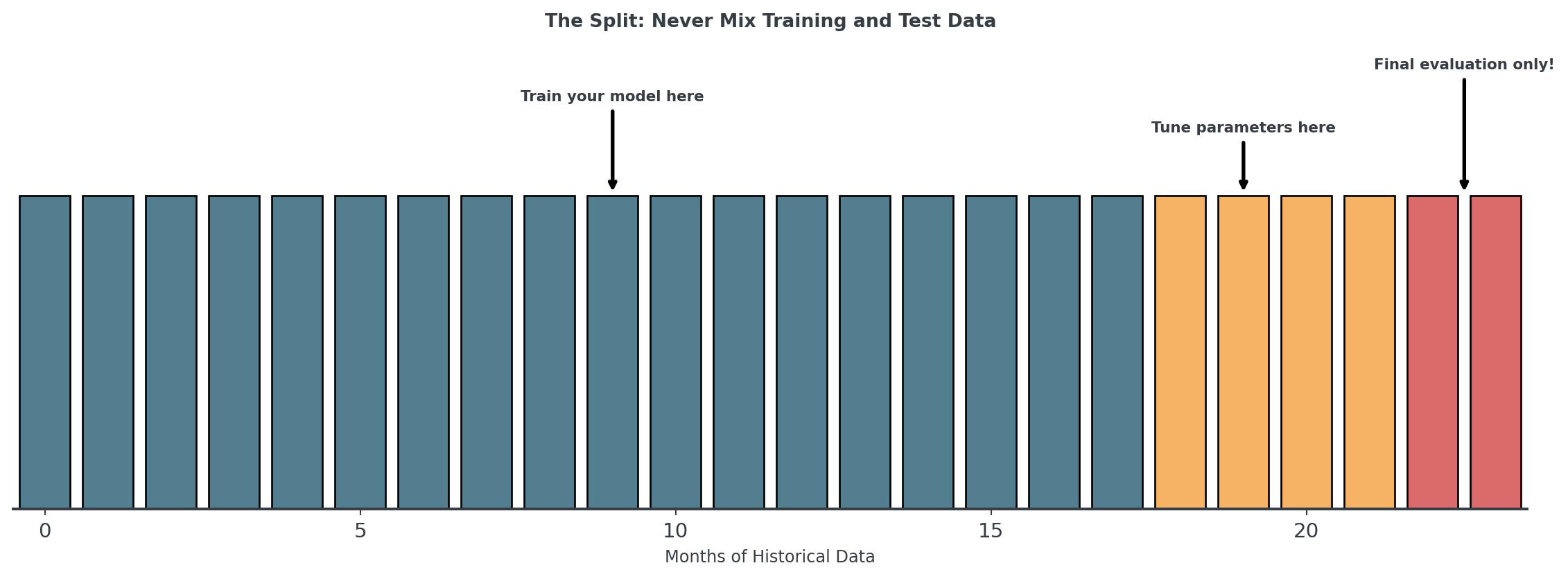
Training Data: Where the model learns patterns (70-80%)
Validation Data: Where you tune hyperparameters (10-15%)
Test Data: The “future”, only once for final evaluation (10-15%)

Data Leakage: The Silent Problem

When future information sneaks into your training data

Target leakage
- Wrong: Including “total_sales” when predicting “monthly_sales”
- Right: Only use information available at prediction time
Temporal leakage
- Wrong: Random split for time series (mixes past and future)
- Right: Always split chronologically

Data leakage can make a terrible model look amazing… until it fails in production!

Time Series Cross-Validation

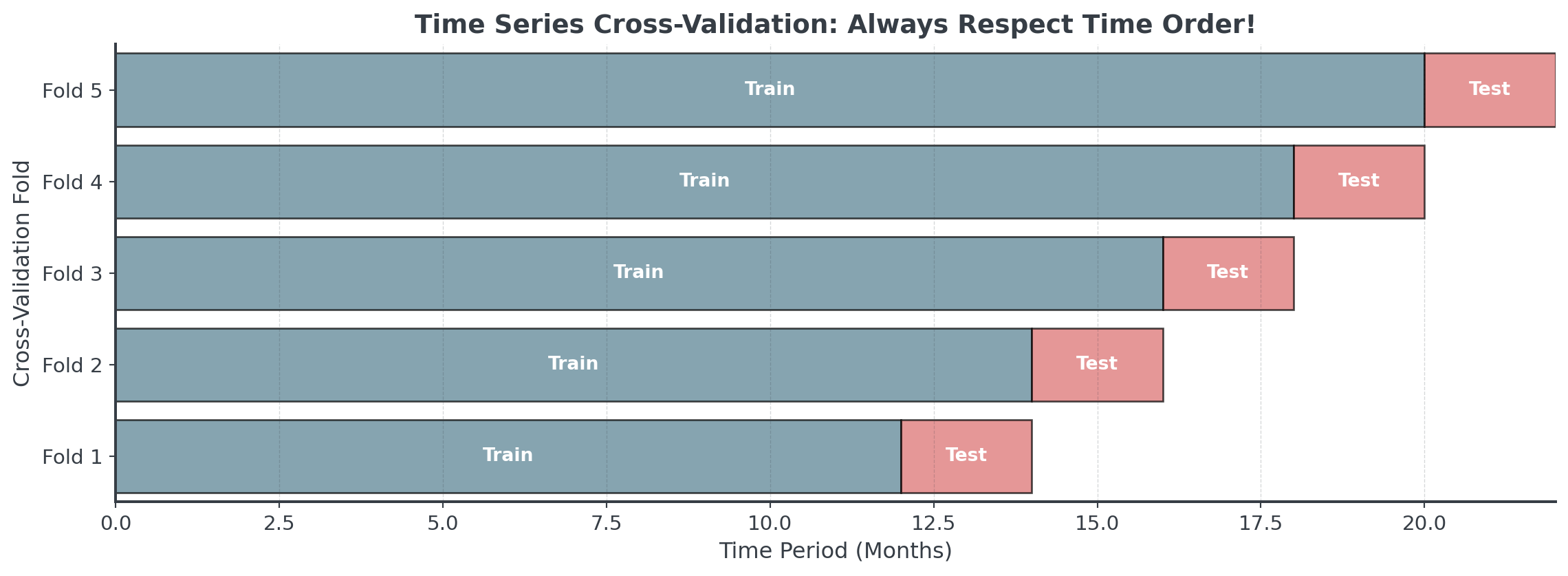
Unlike regular cross-validation, we NEVER use future data to predict the past!

When to Use AI/ML Forecasting I

Use AI when you have:

Sufficient historical data (2+ years)
Rich feature data (weather, promotions, events)
Non-linear patterns
Resources for training/maintenance

Examples:

Large retailers (Amazon, Walmart)
Demand forecasting with many variables

When to Use AI/ML Forecasting II

Don’t use AI when you have:

Limited historical data
High noise, low signal
Need explainable forecasts
Limited expertise

Examples:

New products (no history)
Regulatory environments

Advanced Topics

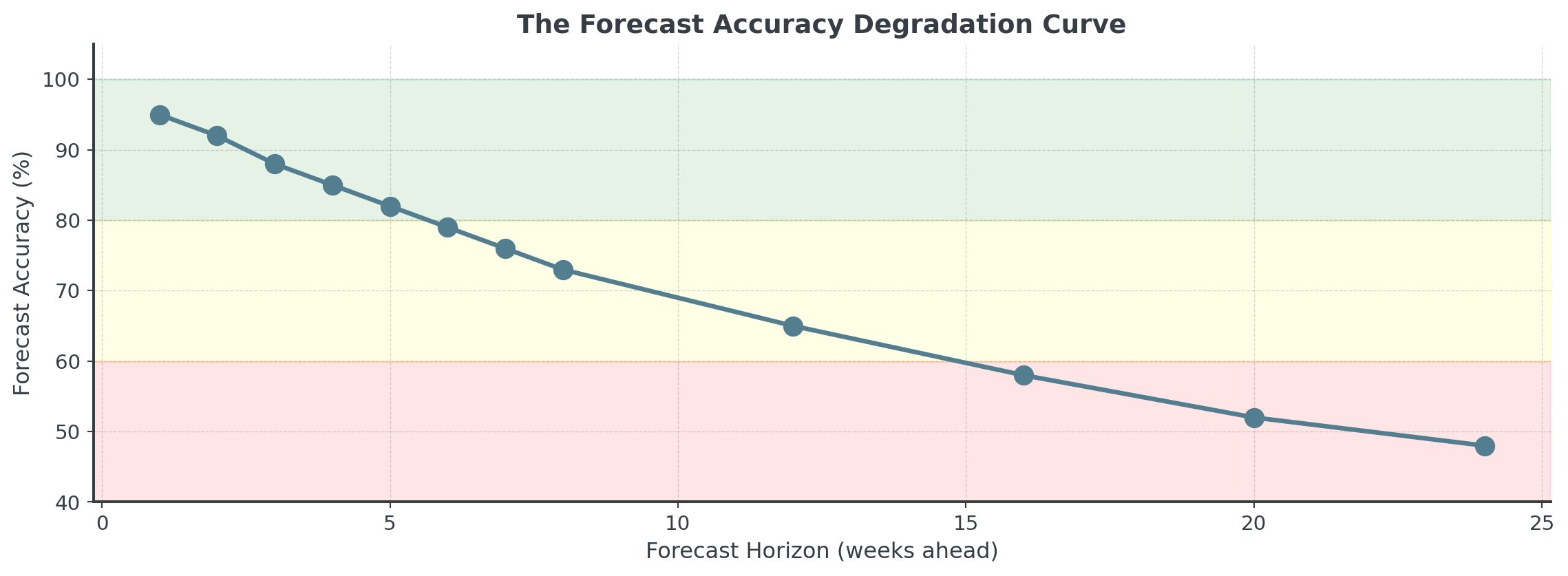
Forecast Horizons

How far into the future can we predict?

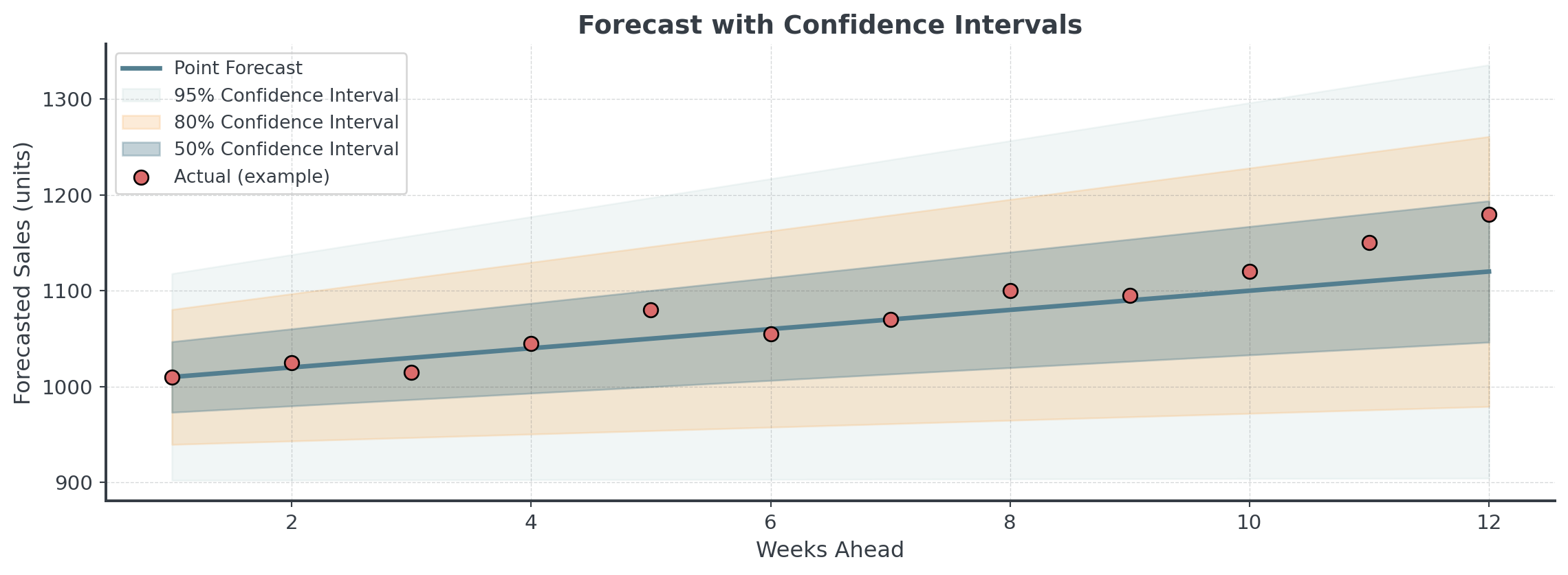
Confidence Intervals

A forecast without confidence intervals is incomplete!

Forecast Combination

Why choose one method when you can combine several?

# Example: Combining multiple forecasts
ma_forecast = 120      # Moving average prediction
exp_forecast = 125     # Exponential smoothing prediction
seasonal_forecast = 135 # Seasonal model prediction

# Simple average (equal weights)
simple_combo = (ma_forecast + exp_forecast + seasonal_forecast) / 3
print(f"Simple combination: {simple_combo:.0f} units")

# Weighted average (based on historical accuracy)
weights = [0.3, 0.5, 0.2]  # Exp smoothing was most accurate historically
weighted_combo = (ma_forecast * weights[0] +
                  exp_forecast * weights[1] +
                  seasonal_forecast * weights[2])
print(f"Weighted combination: {weighted_combo:.0f} units")

Simple combination: 127 units
Weighted combination: 126 units

Lead Times and Safety Stock

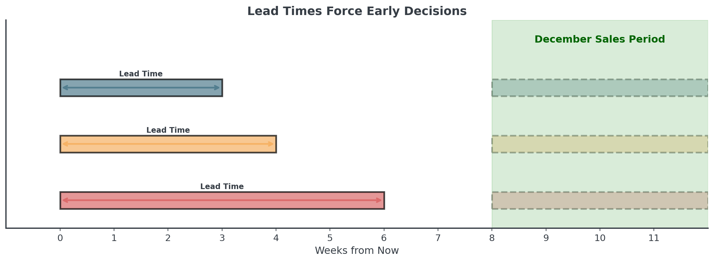
Long lead times = Forecasting further out = Less accuracy = More safety stock!

Safety Stock Calculation

How much buffer do you need?

# Safety stock formula
import scipy.stats as stats

avg_weekly_demand = 300; std_weekly_demand = 40; lead_time_weeks = 3
service_level = 0.95  # Want 95% availability

# Z-score for 95% service level
z_score = stats.norm.ppf(service_level)

# Safety stock calculation
safety_stock = z_score * std_weekly_demand * np.sqrt(lead_time_weeks)
reorder_point = (avg_weekly_demand * lead_time_weeks) + safety_stock

print(f"Average demand during lead time: {avg_weekly_demand * lead_time_weeks} units")
print(f"Safety stock needed: {safety_stock:.0f} units")
print(f"Reorder point: {reorder_point:.0f} units")

Average demand during lead time: 900 units
Safety stock needed: 114 units
Reorder point: 1014 units

Today’s Tasks

Today

Hour 2: This Lecture

Patterns & decomposition
Simple ES, Holt’s, Holt-Winters
Method selection
Practical pandas

Hour 3: Notebook

Bean Counter CEO
Daily and weekly aggregation
Implement methods
Compare accuracy

Hour 4: Competition

MegaMart challenge
3 real products
4-week forecast
€10K per error unit!

The Competition Challenge

“The Christmas Predictor”

Analyze 2 years of weekly sales for 3 products
Identify patterns (trend, seasonality, volatility)
Forecast 4 December weeks for each product
Minimize Mean Absolute Error across all 12 predictions

Key Takeaways

Remember This!

The Rules of Forecasting

Always plot first - Your eyes catch patterns algorithms miss
Start simple - Complexity is not your friend
Recent matters more - Weight recent data higher
Match method to pattern - Trend? Seasonality? Match!
Validate on holdout - Never test on training data
Add confidence intervals - Uncertainty is information
Consider business context - Cost of errors matters

Final Thought

Forecasting is both art and science

The Science:

Statistical methods
AI based forecasting
Error metrics (MAE, RMSE)
Confidence intervals
Systematic validation

The Art:

Choosing the right method
Balancing complexity vs simplicity
Interpreting context
Communicating uncertainty

Make better decisions, not perfect predictions!

Break!

Take 20 minutes, then we start the practice notebook

Next up: You’ll become Bean Counter’s forecasting expert, preparing for seasonal demand!

Then: The MegaMart Christmas Challenge!