Session 07-01 - Descriptive Statistics Essentials

Section 07: Probability & Statistics

Dr. Nikolai Heinrichs & Dr. Tobias Vlćek

Entry Quiz - 10 Minutes

Quick Review from Section 06

Test your understanding of Integration

Find \(\int x \cdot e^x \, dx\) using integration by parts.
Evaluate \(\int_0^1 (2x + 1) \, dx\)
A company’s marginal profit is \(MP(x) = 60 - 2x\). Find the profit function if \(P(0) = -100\).
Find the area between \(y = x\) and \(y = x^2\) from \(x = 0\) to \(x = 1\).

Homework Discussion - 12 Minutes

Your Questions from Section 06

Bring up anything unclear from integration and applications.

Integration by parts setup choices
Definite integral sign mistakes
Area between curves setup
Interpreting marginal functions in business tasks

Today we switch from calculus to data description, but we still need the same habits: clear setup, careful notation, and interpretation in context.

Welcome to Probability & Statistics!

New Section Overview

Session 07-01: Descriptive Statistics (today)
Session 07-02: Basic Probability Concepts
Session 07-03: Combinatorics & Counting
Session 07-04: Conditional Probability
Session 07-05: Bayes’ Theorem
Session 07-06: Contingency Tables
Session 07-07: Binomial & Geometric Distributions
Session 07-08: Mock Exam 2

Probability accounts for approximately 25% of the Feststellungsprüfung!

Learning Objectives

What You’ll Master Today

Calculate measures of central tendency: mean, median, mode
Compute measures of spread: range, variance, standard deviation
Interpret data distributions using histograms and box plots
Work with frequency distributions and relative frequencies
Apply statistical concepts to business scenarios
Understand the normal distribution and the 68-95-99.7 rule

This is foundational material - brief coverage to prepare for probability!

Part A: Measures of Central Tendency

The Three Averages

How do we summarize a data set with a single number?

Three Measures of Center

Mean (Mittelwert): \(\bar{x} = \frac{\sum x_i}{n}\)
Median (Zentralwert): Middle value when data is sorted
Mode (Modalwert): Most frequently occurring value

I’ll figure you already know what these are, but let’s do an example

Example: Sales Data

Monthly sales (in thousands €) for a store:

\(12, 15, 14, 18, 15, 22, 15, 16, 14, 19\)

Question: What is the mean, median, and mode of the data?

Mean: \(\frac{12 + 15 + 14 + 18 + 15 + 22 + 15 + 16 + 14 + 19}{10} = \frac{160}{10} = 16\)

Median: Sort and then the middle values: \(\frac{15 + 15}{2} = 15\)

Mode: \(15\) (appears 3 times)

Easy, right?

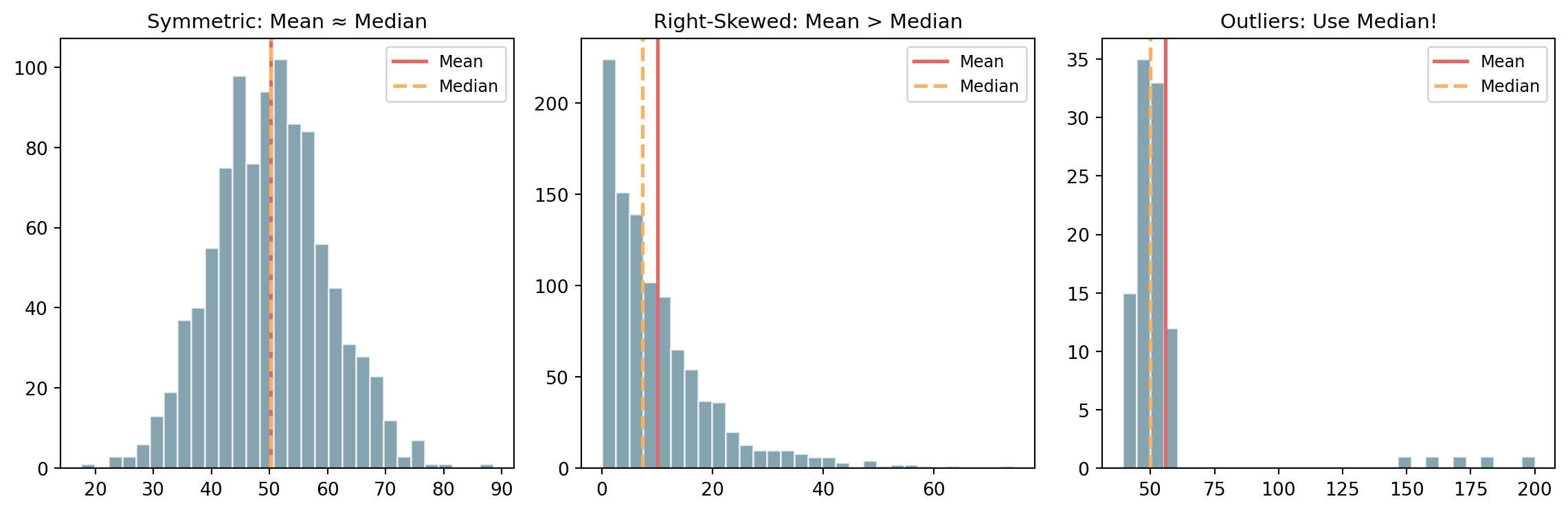
When to Use Each Measure

Mean: Best for symmetric data without outliers; Median: Best for skewed data or data with outliers; Mode: Best for categorical data

Part B: Measures of Spread

How Spread Out Is the Data?

Two datasets can have the same mean but different spreads:

Dataset A: \(48, 49, 50, 51, 52\) (mean = 50)
Dataset B: \(10, 30, 50, 70, 90\) (mean = 50)
We need measures to quantify this difference!

Question: Do you know any measures of spread?

Range

Simplest measure of spread:

\(\text{Range} = \text{Maximum} - \text{Minimum}\)
Dataset A: Range \(= 52 - 48 = 4\)
Dataset B: Range \(= 90 - 10 = 80\)

Range only uses two values - sensitive to outliers!

Outliers are extreme values that are far from other observations.

Variance and Standard Deviation

Used to measure spread around the mean:

They tell us how far the data is from the mean
They are always non-negative

Population variance
Sample variance
Standard Deviation

Used to compute the population standard deviation.

\[\sigma^2 = \frac{\sum (x_i - \mu)^2}{N}\]

Used to compute the standard deviation of a sample.

\[s^2 = \frac{\sum (x_i - \bar{x})^2}{n - 1}\]

The standard deviation is the square root of the variance.

\[\sigma = \sqrt{\sigma^2} \quad \text{or} \quad s = \sqrt{s^2}\]

Calculation Example

Data: \(4, 8, 6, 5, 3, 2, 8, 9, 2, 5\) (n = 10)

Step 1: Calculate mean \[\bar{x} = \frac{4+8+6+5+3+2+8+9+2+5}{10} = \frac{52}{10} = 5.2\]

Step 2: Calculate deviations squared \[(4-5.2)^2 + (8-5.2)^2 + ... = 1.44 + 7.84 + ... = 57.6\]

Step 3: Variance and SD \[s^2 = 57.6/9 = 6.4 \quad \Rightarrow \quad s = \sqrt{6.4} \approx 2.53\]

Part C: Frequency Distributions

Organizing Data

Raw data: Test scores of 30 students

\(65, 72, 78, 81, 65, 73, 85, 92, 78, 72,\)

\(65, 88, 91, 73, 78, 82, 76, 72, 85, 78,\)

\(65, 73, 82, 79, 88, 73, 78, 85, 92, 78\)

Question: How can we summarize this data effectively?

We can use a frequency table or a histogram!

Frequency Table

A frequency table organizes data into groups (bins):

Score Range	Frequency	Relative Frequency
60-69	4	4/30 = 13.3%
70-79	14	14/30 = 46.7%
80-89	9	9/30 = 30.0%
90-99	3	3/30 = 10.0%
Total	30	100%

Relative frequency = Frequency / Total = Probability interpretation!

Histogram Visualization

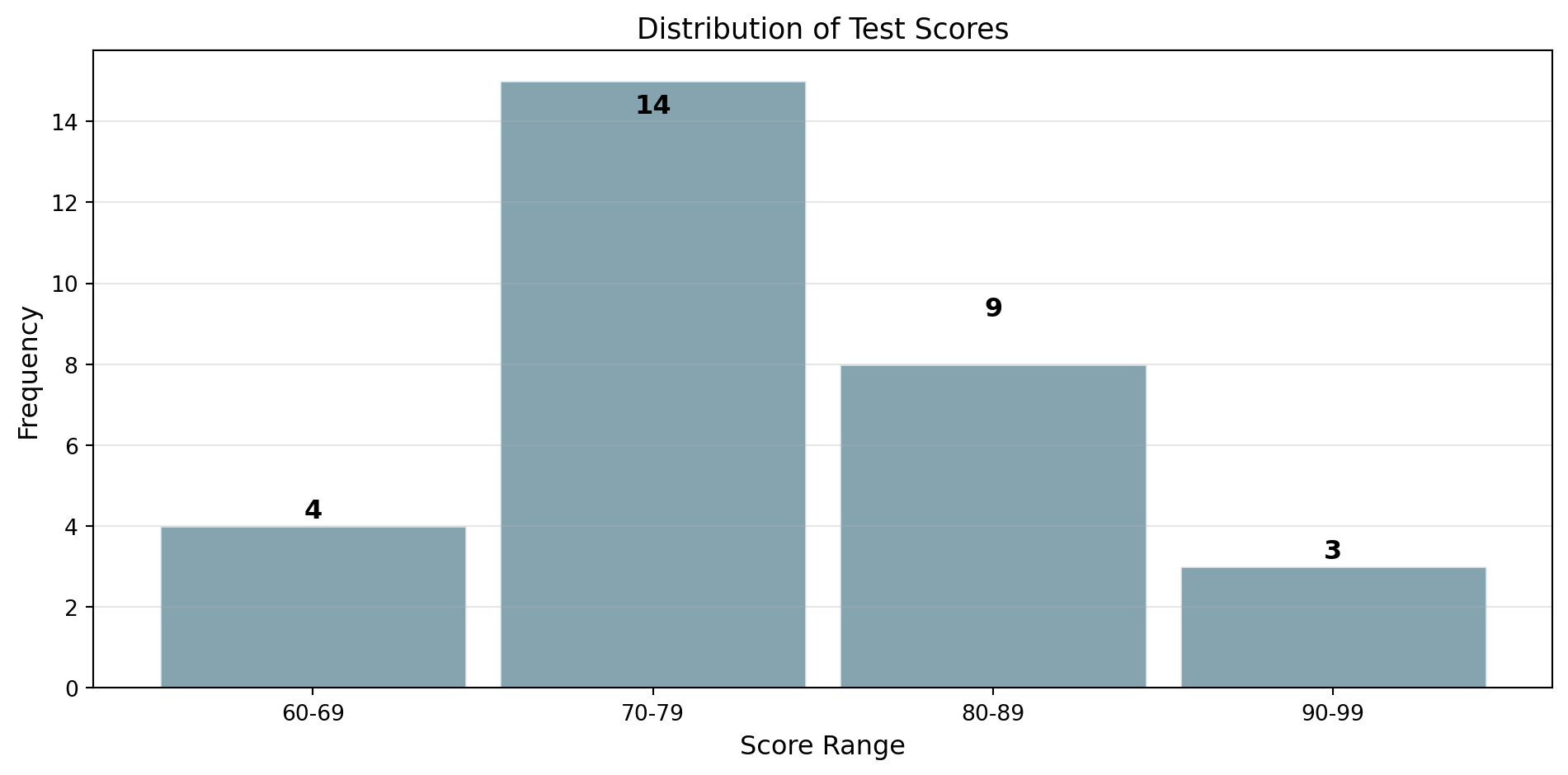
A histogram is a graphical representation of the distribution of data. It is an estimate of the probability distribution of a continuous variable.

Quick Check - 6 Minutes

Quick Check Before the Break

Work individually

For data \(4, 5, 6, 6, 7, 20\), compute mean and median.
Which measure (mean or median) is more appropriate here? Explain in one sentence.
A class has score frequencies: 50-59: 2, 60-69: 5, 70-79: 9, 80-89: 4. What is the relative frequency of 70-79?

Break - 10 Minutes

Part D: Box Plots (Five-Number Summary)

Quantiles and Quartiles

Quantiles divide sorted data into equal-sized groups:

The median is the quantile that splits data into two equal halves (50%)
Percentiles divide data into 100 equal parts (e.g., the 90th percentile)
Quartiles divide data into four equal parts (25% each)

Quartile	Percentile	Meaning
Q1	25th	25% of values fall below Q1
Q2	50th	50% of values fall below Q2 (= Median)
Q3	75th	75% of values fall below Q3

Quartiles are the most commonly used quantiles in descriptive statistics!

The Five-Number Summary

Provides a concise overview of a dataset’s distribution:

Minimum (Min)
First Quartile (Q1) - 25th percentile
Median (Q2) - 50th percentile
Third Quartile (Q3) - 75th percentile
Maximum (Max)

Interquartile Range (IQR): \(\text{IQR} = Q3 - Q1\), contains the middle 50% of the data!

A box-plot can be used to visualize the five-number summary! Let’s take a look at one.

Box Plot Visualization

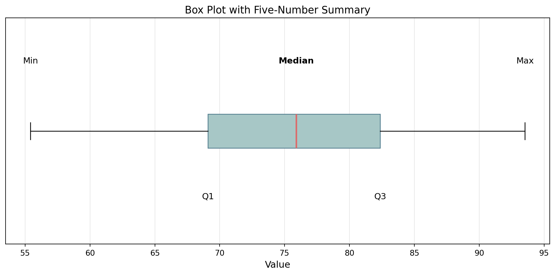
Standardized way of displaying the distribution of data based on the five-number summary!

Detecting Outliers

Outliers are values that fall outside:

The interquartile range (IQR) is the distance between the first and third quartiles.
\(\text{Lower fence: } Q1 - 1.5 \times \text{IQR}\)
\(\text{Upper fence: } Q3 + 1.5 \times \text{IQR}\)
Example: If \(Q1 = 65\), \(Q3 = 85\), then IQR \(= 20\)
- Lower fence: \(65 - 1.5(20) = 35\)
- Upper fence: \(85 + 1.5(20) = 115\)

Any value below 35 or above 115 would be an outlier.

Part E: Normal Distribution Basics

The Bell Curve

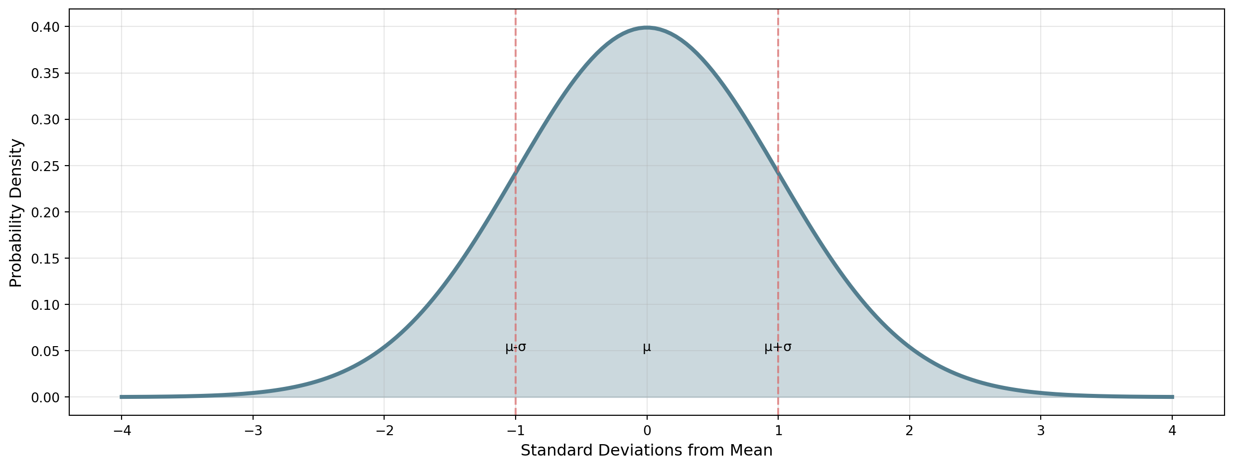
If the data is normally distributed, then: 68% of data falls within \(\mu \pm 1\sigma\); 95% of data falls within \(\mu \pm 2\sigma\); 99.7% of data falls within \(\mu \pm 3\sigma\)

The 68-95-99.7 Rule

Example: Test scores have \(\mu = 75\) and \(\sigma = 10\)

68% of students score between 65 and 85
95% of students score between 55 and 95
99.7% of students score between 45 and 105

Based on the assumption that data is normally distributed, we can make informed guesses about certain things. We’ll see later what this allows us to do in the context of a business application.

Part E: Business Applications

Quality Control: Setup

A factory measures the diameter of manufactured bolts (in mm):

\[10.2, \; 10.1, \; 10.0, \; 10.3, \; 9.9, \; 10.1, \; 10.0, \; 10.2, \; 10.1, \; 10.0\]

Target: 10.0 mm with tolerance ±0.3 mm (acceptable: 9.7 – 10.3 mm)

Task: Compute the mean, median, and mode.

Mean: \(\bar{x} = \frac{10.2 + 10.1 + 10.0 + \ldots + 10.0}{10} = \frac{100.9}{10} = 10.09\) mm
Median: Sorted middle values: \(\frac{10.1 + 10.1}{2} = 10.10\) mm
Mode: \(10.0\) mm (appears 3 times)

The mean (10.09) exceeds the target (10.0), indicating a slight upward bias in production.

Quality Control: Spread

Same data: \(10.2, \; 10.1, \; 10.0, \; 10.3, \; 9.9, \; 10.1, \; 10.0, \; 10.2, \; 10.1, \; 10.0\)

Task: Compute range, sample variance, and sample standard deviation.

Range: \(10.3 - 9.9 = 0.4\) mm
Sample variance: \(s^2 = \frac{\sum(x_i - \bar{x})^2}{n-1} = \frac{0.129}{9} \approx 0.014\)
Standard deviation: \(s = \sqrt{0.014} \approx 0.12\) mm

The standard deviation (0.12 mm) is small relative to the tolerance (±0.3 mm) and the target (10.0 mm). This suggests the process has low variability!

Quality: Five-Number Summary

Task: Sort the data and find the five-number summary and IQR.

Sorted: \(9.9, \; 10.0, \; 10.0, \; 10.0, \; 10.1, \; 10.1, \; 10.1, \; 10.2, \; 10.2, \; 10.3\)

Measure	Value
Min	9.9
Q1	10.0
Median	10.1
Q3	10.2
Max	10.3

\(\text{IQR} = Q3 - Q1 = 10.2 - 10.0 = 0.2\) mm

Quality Control: Outlier Detection

Task: Compute the fences and check for outliers.

\(\text{Lower fence} = Q1 - 1.5 \times \text{IQR} = 10.0 - 1.5 \times 0.2 = 9.7 \text{ mm}\)
\(\text{Upper fence} = Q3 + 1.5 \times \text{IQR} = 10.2 + 1.5 \times 0.2 = 10.5 \text{ mm}\)
All values fall within \([9.7, \; 10.5]\)
→ no outliers detected!

The tolerance is \([9.7, \; 10.3]\) mm. The upper fence is slightly above the upper tolerance limit, but since no values exceed the tolerance, we do not have to worry about outliers.

Quality Control: Normal Distribution

Task: Assuming normality with \(\bar{x} = 10.09\) and \(s = 0.12\), compute the 68-95-99.7 intervals. Do all fall within the tolerance \([9.7, \; 10.3]\)?

Rule	Interval	Within tolerance?
68%	\([10.09 \pm 0.12]\)	Yes
95%	\([10.09 \pm 0.24]\)	No — upper end exceeds 10.3
99.7%	\([10.09 \pm 0.36]\)	No — upper end clearly outside

About 95% of bolts are expected within tolerance, but the upper tail extends beyond the 10.3 mm limit due to the upward-shifted mean.

Keep in mind that we only have \(n = 10\) measurements, with such a small sample, the 68-95-99.7 rule is only a rough approximation. Larger samples give more reliable estimates of \(\bar{x}\) and \(s\).

Quality Control: Business Decision

Task: Should the factory manager be concerned?

Summary of findings:

Mean is above target: \(10.09 > 10.0\) (upward bias)
Low variability: \(s = 0.12\) mm (good precision)
No outliers in the current sample
But the 95% interval \([9.85, \; 10.33]\) exceeds the upper tolerance
Potential cause: the machine is precise but not accurate!

Recommendation: Recalibrate the machine to shift the mean closer to 10.0 mm. The low standard deviation means the process only needs recentering, not a reduction in variability.

Guided Practice - 15 Minutes

Practice Problems

Work in pairs for 5 minutes

Problem 1: Customer wait times (minutes): \(3, 5, 2, 8, 4, 6, 3, 7, 2, 10\)

Calculate mean, median, and mode
Calculate variance and standard deviation
Is the mean or median a better measure of center? Why?

Problem 2: Create a frequency table for exam scores:

\(75, 82, 91, 78, 85, 68, 73, 88, 95, 79, 82, 76, 84, 90, 77\)

Chained Exam Mini-Problem

Work individually, then compare

A shop tracks daily visitors and purchases:

Of 250 visitors, 65 make a purchase. Estimate purchase probability \(p\).
Using your result, estimate expected purchases for 400 visitors.
If actual purchases are 88, compare actual vs expected and interpret in one sentence.

Coffee Break - 10 Minutes

Collaborative Problem-Solving - 20 Minutes

Store Performance Dashboard

Think individually, then work in groups of 3-4 and share

A retail manager reports weekly sales (in thousand euro):

\[41, 44, 43, 45, 46, 47, 44, 90\]

Compute mean, median, range, and sample standard deviation.
Identify whether there is an outlier signal and justify using IQR logic.
Recommend which center measure should be shown on the dashboard.
Write a two-sentence business interpretation for management.

Connection to Probability

From Statistics to Probability

Key connection:

\[\text{Relative Frequency} \approx \text{Probability}\]

Example: If 30% of customers wait more than 5 minutes, then the probability that a randomly selected customer waits more than 5 minutes is approximately 0.30.

This is the frequentist interpretation of probability, which states that probability equals long-run relative frequency!

Final Assessment - 5 Minutes

Exit Assessment

Work individually

For data \(2, 4, 4, 5, 100\), should you report mean or median as the typical value?
Explain the difference between variance and standard deviation in one sentence.
If 18 out of 60 customers choose option A, what is the relative frequency?

Wrap-Up & Key Takeaways

Today’s Essential Concepts

Mean, median, mode measure center differently
Variance and standard deviation measure spread
Box plots show distribution shape and outliers
Normal distribution: 68-95-99.7 rule for bell curves
Relative frequency connects to probability
Choose the right measure based on data characteristics

Next Session Preview

Coming Up: Basic Probability Concepts

Sample spaces and events
Probability axioms and rules
Complement and addition rule
Independent vs mutually exclusive events

Homework

Complete Tasks 07-01:

Calculate descriptive statistics for business datasets
Interpret measures in context
Prepare for probability concepts